Sage Journals: Discover world-class research

Abstract

The principle of the thread fastenings have been known and used for decades with the purpose of joining one component to another. Threaded fastenings are popular because they permit easy disassembly for maintenance, repair, relocation and recycling. Screw insertions are typically carried out manually. It is a difficult problem to automat. As a result there is very little published research on automating threaded fastenings, and most research on automated assembly focus on the peg-in-hole assembly problem. This paper investigates the problem of automated monitoring of the screw insertion process. The monitoring problem deals with predicting integrity of a threaded insertion, based on the torque vs. insertion depth curve generated during the insertions. The authors have developed an analytical model to predict the torque signature signals during self-tapping screw insertions. However, the model requires parameters on the screw dimensions and plate material properties are difficult to measure. This paper presents a study on on-line identification during screw fastenings. An identification methodology for two unknown parameter estimation during a self-tapping screw insertion process is presented. It is shown that friction and screw properties required by the model can be reliably estimated on-line. Experimental results are presented to validate the identification procedure.

Keywords

threaded fastenings screw insertions Newton Raphson Method two unknown estimations parameter estimations autonomous threaded assembly autonomous process system

1. Introduction

Screw insertions are a common joining process and are especially popular in assemblies that need to be disassembled for repair, maintenance or relocation.

A human performing screw fastening will typically use four stages (L.D. Seneviratne, F.A. Ngemoh and S.W.E. Earles, 1992): 1)

Alignment: the holes in the mated parts are aligned and firmly held together.

Positioning: the screw is globally positioned with respect to the aligned holes.

Orientation: the screw is oriented until its axis coincides with the axis of the aligned holes.

Turning: the screw is turned with the appropriate torque until fastening is achieved.

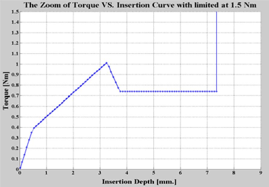
In manual screw insertions, the torque exerted by the screwdriver depends mainly on the applied operator force. Human operators are particularly good at on-line monitoring of the operation. However, with power tools, the increased insertion speed reduces the human ability to monitor the insertions on-line. Thus on-line automated monitoring strategies for the screw fastening process are highly desirable. One such approach is based on the “Torque Vs. Insertion Depth” signal measured in real time; if this signal is within a pre-defined bound of the correct insertion signal, then the insertion is considered to be satisfactory. The torque signature signal for a correct insertion is either taught as predicted using an analytical model (M. Klingajay, L. D. Seneviratne, 2002).

Industrial applications of automated screw insertions have been implemented in several forms. These achieved forms are applied in different objectives. With the development of electrically powered screwdrivers the attempts at automating the screw insertion process with emphasis on the torque signature signal vs. angle signal and become to the primary mathematical model. In 1997, this analytical model was implemented by (F.A. Ngemoh, 1997). The Neural Network techniques have been applied by using the ability of Weightless to monitor the screw insertion processes in difference insertion cases (Visuwan P., 1999). Bruno has distinguished between successful and unsuccessful insertion based on Radial Basic function (Bruno Lara Guzman, 2000). Both monitoring performs are to apply Artificial Neural Network in view points of classifications.

“A distinction without a difference has been introduced by certain writers who distinguish ‘Point estimation’, meaning some process of arriving at an estimate without regard to its precision, from ‘Interval estimation’ in which the precision of the estimate is to some extent taken into account” (Fisher, R. A., 1959).

Fisher founded the Probability theory as logic agree, which gives us automatically both point and interval estimates from a single calculation. The distinction commonly made between hypothesis testing and parameter estimations are considerably greater than that which concerned Fisher. In this point of view, it may be not a real difference.

The screw fastening processes have carried out insertion on eight different materials of plate and the general self-tapping screws with using mainly screw sizes AB No. 4, No. 6, and No.8. These self-tapping screw sizes are the most common sizes in manufacturing.

The corresponding theoretical profiles of a curve of the torque signature signal and rotation angle for each set of insertions have been also generated using the mathematical model by (L.D. Seneviratne, F.A. Ngemoh, S.W.E. Earles, and K. Althoefer, 2001). The mechanical properties of the plate materials have used the theoretical model that was obtained from (F.A. Ngemoh, 1997). The average properties have used the provided data sheets that were the published texts and materials standards specifications (ASM V.1, 1990); (ASM V.2, 1990); and (C. H. Verlag, 1993); (R. A. Walsh, 1993); and (D. Bashford, 1997).

2. The experimental test rig setup

The Implementation of Screw Insertion System model (ISIS) has been integrated with three main factors. The first one is the screwdriver with the pilot materials for attempt to insertion screw. The second one is the instruments and sensor controller. This controller consists of the Rotary transducer or Torque sensor for capture a torque signature signal and the Optical Encoder for measurement the rotation angle during the on-line process. This controller is including the torque meter and manipulator equipments. The third one is the monitoring system based-on the parameter estimation has employed for prediction of the required parameters of the threaded fastening process. These factors have interfaced and implemented by the Graphical User Interface technique (GUI) using Matlab programming. More details on these equipments have described in next.

2.1. Tools and manipulations

The tools and manipulations are necessary as input devices, which brought the input signal to the process. An electrically powered screwdriver has used with a torque range varying from 0.4 to 3.2 Nm to drive the screw into the hole for this experimental testing. An illustration this screwdriver present in Fig. 1.

Fig. 1

The illustration of screwdriver

2.2 The instrument and sensor controller

The controller is main function to command the process that aims to control the instruments and sensors for the on-line operation. The integrated fastening process with GUI system has been employed and interfaced with the Data Acquisition (DAQ) card. The details of these devices are following.

2.2.1 Torque Transducer or Torque Sensor.

In Fig. 2, the rotary torque transducer has used in this experiment, which has attached to the shaft of the screwdriver between the end of screwdriver and the nut settings. This torque sensor is in position that can reduce the effects of inactive and friction associated of the gear and the drive motor and gears. This torque sensor is a measurement based on strain gauges with capable in measuring torque is in the range between 0 and 10 Nm with accuracy of 1% of full scale deflection.

Fig. 2.

Torque Sensor.

The Torque sensor was electronically interfaced with a digital torque meter that is produced and used of a strain gauge amplifier. The voltage output of torque reading from the torque meter is proportional to the measured torque during screw insertion into the hole. Each output voltage has corresponded to the maximum transducer capacity of torque at 10 Nm.

2.2.2 Optical Encoder

An optical encoder has used to measure the rotation angle of the screw. This optical encoder consists of an optical switch and a measured disc. The optical switch has functioned with a light sensitive device with a built-in amplifier, the shape and wiring diagram are presented in Figs. 3 and 4. It was mounted on the torque sensor casing. The optical switch used in this test to be model of UZJ272. Its performance is to fix-focus reflective/u-shaped type micro-photosensors low-cost performance, it is stable detected by fixed-focus reflective.

Fig. 3.

The application of Optical Encoder

Fig. 4.

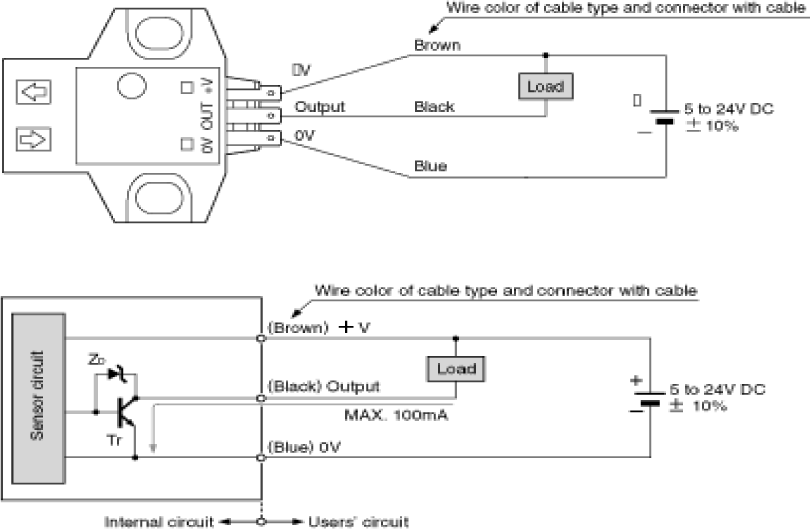
Typical wiring diagrams

A measurement disc has attached to the Torque sensor, which fixed at the shaft of the driver bit see Figs 2 and 4. This disc is perforated every 45° allowing 8 readings per revolution. Every time a hole in the plate is detected the opto-switch produces a voltage pulse by measurement strategy in Fig. 5.

Fig. 5.

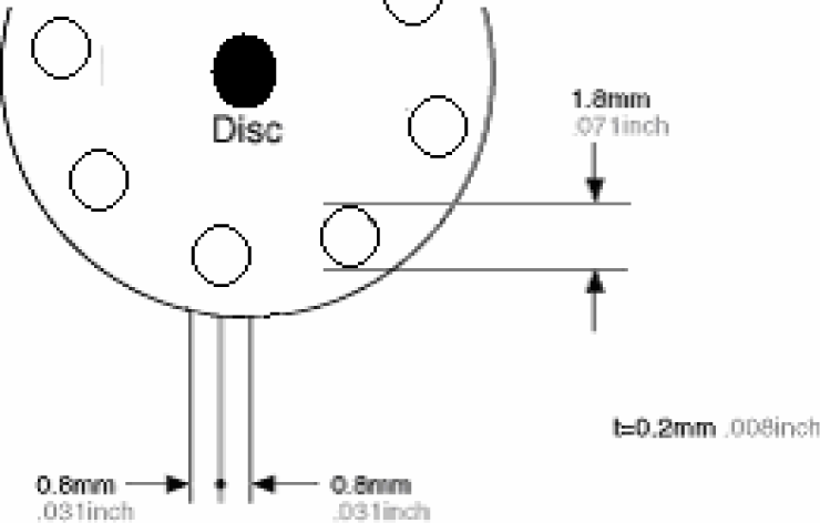
A measurement disc

The Optical encoder has a measurement resolution of 45°. This digital signal of a pulse voltage has been converted to the rotation angle (radial) during screw insertion. This application for reading signal on 8 holes as angle has present in Fig. 6.

Fig. 6.

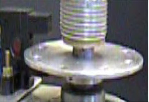
Optical Encoder (Opto switch and Disc)

2.2.3 The reference label box or connector box

This reference label box is used to select the channel, port number, and type of signal for system to identify during on-line process. This box has connected with the SH68-68 cable to the Multifunction DAQ card see Figs. 7 and 8. The details of the Multifunction DAQ card has described in next.

Fig. 7.

The wiring circuit in the Connector box.

Fig. 8 (a).

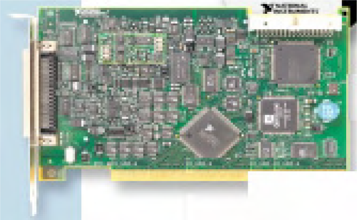
A multifunction DAQ PCI card.

2.2.4 A Multifunction DAQ card.

The multifunction DAQ 12 Bit Analog-Digital I/O card has used in this experimental test is product of National Instrument and Sensor (NI) with model “NI PCI 6024E”. This is required as PCI bus, which is the low-cost E Series multifunction data acquisition device. It provides the full functionality of I/O 68-pin male 0.050 D-type with voltage output range of ± 10 volts.

A multifunction DAQ card in Figs. 8 (a)–(b) have connected the SH68-68 cable and fixed into PCI slot on computer board.

The screwdriver attached the instruments with sensor controllers for this experimental test, shown in Fig. 9. The integrated component system (hardware) has applied for this experimental test of screw fastening system, which shown in Fig. 10.

Fig. 8 (b).

NI DAQ PCI 6024E card with application

Fig. 9.

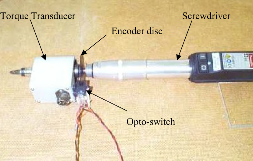
A screwdriver attached transducer and encoder

Fig. 10.

The screw fastening setup

3. Strategy for the on-line experimental test

The experimental equipments are required to connect as the applied screw fastening software has implemented as the appropriated efficiency system with this integrated system has written using Graphic User Interface format (GUI) and Data Acquisition Toolbox of Matlab program to get signal from the torque sensor and optical encoder for Torque signature signal and rotation angle during the screw insertion. The captured signal has been applied the curve fitting and curve management techniques to identify the curve. The parameter estimation method has used the identified curve to predict the unknown parameters at these insertions at stage 2, 4, and 5. The details have presented the flowchart in Fig. 11.

Fig. 11.

Flowchart of the on-line procedures

Fig. 12.

The overview of the experimental test rig

A flowchart in Fig. 11 presents the implemented procedure that applied the DAQ module to communicate between the screwdriver and the instruments and sensors. The performance of the screw insertion identification tasks, the NRM technique is fed with torque-insertion depth signature signals. The screw insertions were performed with the use of a screwdriver. A torque sensor mounted at the tip of the screwdriver provides torque readings, and an optical encoder provides pulses, which are related to the screw rotation angle.

The stream of pulses was integrated to determine the corresponding insertion depth. Model was developed and using the curve fitting technique to filter the signal. The experimental test rig prior to presentation to the on-line screw fastening process for the parameter identification has been described in next. An online screw fastening process software has used to manage all instruments and sensors for the input task and interfacing with the screwdriver and linking with the monitoring based-on parameters estimation. The main functions of this control system have been implemented as GUI format.

Reading the torque vs. time data from the torque transducer and the rotation angle vs. time data from the optical encoder. These online results can be presented the signal data in Fig. 13.

Fig. 13.

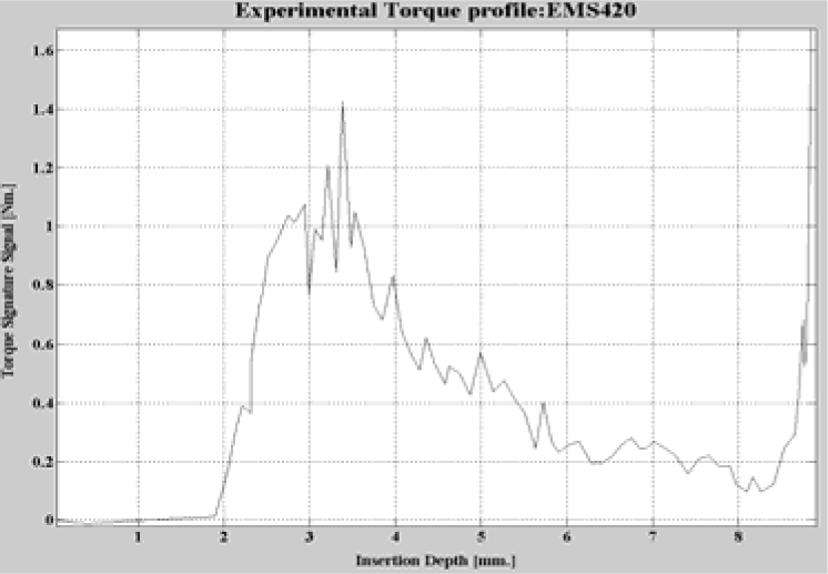
The result from online experimental test.

The curve fitting technique has applied to fit the original signal from the experiment in Fig. 14. This technique has explained for more details in the next section.

Curve management process is the straight line technique to find the slop changing for recognition of the insertion torque at stage 2, 4, and 5. Interfacing the torque-angle curve with the parameters identification monitoring software.

Fig. 14.

The signal fited by the curve fitting technique

In this chapter has used the monitoring technique based on parameter estimation to validate the experimental tests with simulation tests (theoretical model). The parameter estimation based on Newton Raphson Method has used to identify the unknown parameters. This estimation algorithm has applied the torque signature signal and rotation angle signal after fitting the smooth curve. This smooth curve has fitted after the online experimental tests. This curve fitting technique has described in next.

3.1. Curve fitting technique on the experiment

The smooth curve can be fitted and applied to the experimental signal. Using the interpolating polynomial of n^th degree then we can obtain a piecewise use of polynomials, this technique is to fit the original data with the polynomial of degree through subsets of the data points. This result is quite suitable approach as a least square fit algorithm. That has applied these fitting on points with the exactly points so close to actual curve when has been validated with theoretical curve.

Curve fitting to measure the signal data is a frequently occurring problem. These signals are two vectors x and y of equal size. The situation is aims to fit the data because being a dependency of y on x in form of a polynomial. The method of least squares can be used to solve the over constrained linear system which gives the coefficients of the fitting polynomial. Therefore, the higher degree polynomial has represented the dependency for this fitting technique.

For a given data set (x; y) - where x and y are vectors of the same size. The least square technique can be used to compute a polynomial for that best fits these data has used a polyfit function at the degree of the fitted polynomial.

An illustration problem on this technique has applied on experimentally with the relationship between two variables x and y that have recorded in a laboratory experiment in Fig. 15. However, this captured curve has been fitted for a new validated smooth curve with the curve fitting algorithm has described in next.

Fig. 15 (a):

The on-line signal or original curve

In Fig. 15 (a) shows a captured curve from the experimental test during on-line insertion. The curve fitting method has been employed using an algorithm of the polynomial technique is based on Least Square technique has that apply to fit on this captured curve. This a new smooth curve after fitting process has presented in Fig. 15.(b).

Fig. 15 (b):

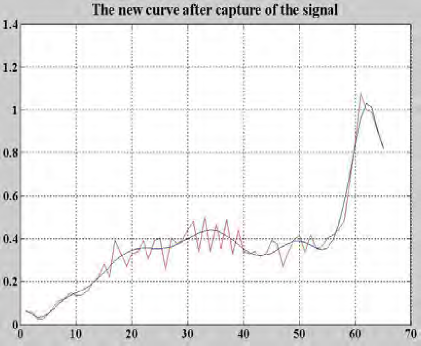
The adjust curve during the curve fitting.

The on-line curve has been adjusted for the actual starting point of insertion then the new smooth fitted curve has presented the experiment torque signature signal in Fig. 15 (c).

Fig. 15 (c):

The new smooth fitted curve.

The validated curve of experimental curve has compared with theoretical curve to be shown in fig. 16.

Fig. 16.

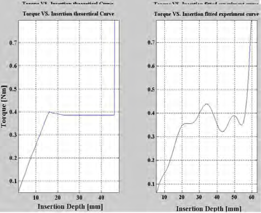
The theoretical and experimental curves.

3.2. The experiment curve identification

The screw insertion process has been described on the required parameters depend on the each equation in the five different stages of insertion. Therefore, this NRM algorithm has applied with screw insertion process that required the exactly Displacement of depth, which has applied for those curves in each stage. Thus, the curve identification technique has become the important technique to employ for recognition the curves of the torque signature signal and displacement of depth of insertion.

Basically, the actual curve of the torque signature signal and rotation angle is the non-linear curve as being discontinue in each stage of insertions. These stages have divided the nature curves that could be generated from simulation tests or captured during experiment tests. Therefore, these parts of curve have be identified by this curve fitting technique for screw fastening process, more details has explained in next.

The screw, material, and plate properties in Table 1 have been used to produce the simulation screw insertion curve in Fig. 16.

Table 1.

Parameters for insertion of Polycarbonate and screw AB 6

Material and hole properties
Material type	Polycarbonate
Thickness	3 mm (0.003 Meters)
Yield strength	45Mpa
Tensile strength	45Mpa
Elastic modulus	2.35Gpa
Coefficient of friction	0.19
Tap hole diameter	2.0 mm (0.0020 Meters)
Near plate thickness	0 (not used)
Screw properties
Type	AB No. 6
Material	Zinc plated steel
Major diameter	3.42mm (0.00342 Meters)
Root diameter	2.49mm (0.00249 Meters)
Pitch	1.19mm (0.00119 Meters)
Length	9.67mm (0.00967 Meters)
Taper length	2.94mm (0.00294 Meters)
Head screw diameter	6.52mm (0.00652 Meters)

Fig. 16.

The curve for screw AB6 with Polycarbonate

This insertion stage is status of the screw makes first contact with the hole wall in the tap plate. This curve has been identified the insertion stage in Figs. 17–19.

Fig. 17.

The identified insertion curve as stage 2

The identified insertion curve at stage 2 has been present in Fig. 17. This curve shows that the curve of the Displacement of depth in stage2.

The torque signal on this curve at stage 4 is straight line. Because this stage is status of Screw sliding, where the screw advances without thread cutting until the screw head contacts the top plate. Therefore, this straight line is an identified curve at stage 4 to be present in Fig. 18. In Fig. 19 shows that the last stage of insertion curve has been identified as the stage 5 of curve. This behaviour presented to status of the screw had been turned until the final tightening torque been reached. These stage curves have used to estimate for the experiment of parameter identification with explanation in next.

Fig. 18.

The identified insertion curve as stage 4

Fig. 19.

The identified screw insertion curve as stage 5

4. Methodology of parameter estimation

In this paper present what is probably the most commonly used techniques for parameter estimation. The appropriable techniques for the particular attention in this paper devote to discussions about the Newton Raphson Methos is a choice of appropriate minimization criteria and the robustness of this application. The monitoring strategies have been applied the parameter estimation techniniques to validate the screw insertion process in this experimental test.

Fig. 20 present the flow chart of the monitoring based on Parameter Estimation process. Ideally, the model will be explaining the mean of the data, i.e. all that is not measurement error. A model is necessary for the mean, one for the error and a way of checking the model goodness of fit, which mean the new appropriate data to fit to the correct process.

Fig. 20:

The flow chart of monitoring

The main contribution of this thesis is to apply the methodology of (dynamic) for the estimated parameter application based on Newton Raphson Method (NRM) for threaded fastening process with testing on the torque signature vs. insertion angle at insertion stage 2.

The model based monitoring has implemented with following the estimation parameters Scheme in Fig. 21. In this Scheme, the required parameters have read the input data with contain both known and unknown parameters. A V vector consists of known parameters, the rotation angle (φ), a torque signature signal (τ), and the unknown parameter is a vector x_n that be initialed value.

Fig. 21.

Estimation Parameters Scheme

5. Analytical Model for Parameter Estimation

The focus on the experimental test parameter estimation based on NRM, which is the non-linear estimation parameter techniques that can solve problem over threaded fastening for screw insertion process. With parameters on the screw properties, plate properties, and material properties including friction, these techniques have been applied to predict two unknown parameters in this paper. These two unknown parameters are required by the mathematical model can be estimated reliably online. experimental results without noise is presented to validate the estimation procedure in this paper. A self-tapping screw geometry and analytical model from Ngemoh (F.A. Ngemoh, 1997) is presented. A general self-tapping screw process is mentioned in (L.D. Seneviratne, F.A. Ngemoh and S.W.E. Earles, 1992) and (M. Klingajay, L. D. Seneviratne, 2002) consist of five equations corresponding to each insertion stage:

τ_{1} = \frac{1}{α} R_{s} A_{c} σ_{U T S} cos θ . φ + μ R_{f} K_{f} σ_{f} cos θ (φ)

(5.1)

τ_{2} = R_{s} A_{c} σ_{U T S} cos θ 2 + μ R_{f} K_{f} σ_{f} cos θ (φ - α)

(5.2)

τ_{3} = \frac{1}{α} R_{s} A_{c} σ_{U T S} cos θ + μ R_{f} K_{f} σ_{f} cos θ (φ_{b} + φ)

(5.3)

τ_{4} = 2 μ R_{f} K_{f} σ_{f} cos θ (φ_{b})

(5.4)

τ_{5} = [(\frac{μ (D_{s h}^{3} + D_{s}^{3})}{3 (D_{s h}^{2} - D_{s}^{2})}) + (\frac{D_{s} + D_{h}}{4}) . (\frac{π μ (D_{s} + D_{h}) + 2 P}{π (D_{s} + D_{h}) - 2 μ P})] . [\frac{K_{t h} K_{t b}}{K_{t h} + K_{t h}}]

Equation 5.1 to 5.5 can be written as

τ = F (X, φ),

(5.6)

Where φ is the screw angular rotation,

X is the vector of system parameters:

X = [D_h, D_r, D_s, D_sh, P, L_s, L_t, T₁, T₂, E, μ, σ_Y, σ_UTS].

Where

D_h = Tap Hole Diameter

D_r = Screw root diameter

D_s = Screw major diameter

D_sh = Screw head diameter

P = Screw thread pitch

L_s = Screw total threaded-length

L_t = Screw taper-length

T₁ = Tap (near) plate thickness

T₂ = Tap (far) plate thickness

E = Elastic Modulus

μ = Coefficient of Friction

σ_Y = Yield Strength

σ_UTS = Tensile Strength

In the equations 5.1 to 5.5, the following variables, [θ, α, β, A_c, φ_b, K_th, K_tb, R_s, R_f, K_f] are all a function of X, and are given in Appendixes.

Thus given the system parameter vector (D_h, D_r, D_s, D_sh, P, L_s, L_t, T1, T₂, E, μ, σ_Y, σ_UTS). These parameters are important parameter that to be both variable and fixed parameters and the set of equations (5.1–5.5) required these parameters and can be used to predict the torque signature signals. The system parameters are discussed in more detail below.

However, these parameters are simply the important factors for the theoretical model. How to efficiently determine the model parameters are part of the prediction process. In the past, little attention has been paid to this important issue. Because the estimated plan is not known until the calculation is done, several manual trial-and-error adjustments of the parameters are often needed to obtain an actually acceptable value. These values could be solved by parameter estimation techniques.

As the torque signature signal at stages 1 and stage 3 is very small value and too difficult to apply. Therefore, the torque signal at stages 2, 4, and 5 are used to investigate in this research. An estimation parameter has been employed to predict the unknown parameters on the torque signature during screw insertion. As the torque signature signals are non-linear, therefore, the technique is applied with the multi-phase regression with all required parameters on the screw properties, plate properties, and material properties, including friction.

To find the estimated parameters, similar methods as described in the introduction to maximum likelihood estimation section in chapter4 can be used. Because of the structure of this problem, numerical methods must be used to iteratively find these estimates. The common methods often used are the Newton-Raphson Method and Least Square Method; these methodologies have been applied to test and compare the appropriate ability on this work on simulation tests and experimental tests. However, these simulation torque signals need to be classified the insertion stages by using identification of curve technique.

This paper has used the mathematical model that is presented in (L.D. Seneviratne, F.A. Ngemoh and S.W.E. Earles, 1992); (L.D. Seneviratne, F.A. Ngemoh, S.W.E. Earles and K. Althoefer, 2001); (Klingajay M., L.D. Seneviratne, 2002). A model of the self-tapping screw fastening process has used the equation of five stages, which are given in Appendix1.

Initially, the stage 2 equations, that is the torque required to drive the screw from screw engagement till initial breakthrough, is used for parameter estimation in equation (5.2) and can be written as

τ_{2} = f (μ, θ, σ_{U T S}, β, φ, D_{s}, D_{h}, L_{t,} P)

(5.7)

In conventional estimation theory, these parameters of screw insertion are generally determined using the technique of numerical method with the initial value and number of independent samples. The field of optimisation is interdisciplinary in nature, and has made a significant impact on many areas of technology. As the result, optimisation is an indispensable tool for many practitioners in various fields. Usual optimisation techniques are well established and widely published in many excellent publishing, magazines, and textbooks depend on their applications. For all their complexity, the algorithms for optimising a multidimensional function are routine mathematical procedures.

An algorithm of Newton-Raphson Method (NRM) has developed and used for inversion purposes is presented. It achieves convergence in about n^th iterations and produces exact values of the parameters depends on the number of unknown parameter that is going to apply. The curves of torque signature and insertion angle signal are simulated using the successful data from Ngemoh [Ngemoh97] to validate in different screw, material, and plate properties. The curves identification and the Newton Raphson Method (NRM) have been explained with two dimensions.

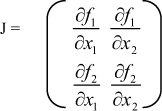
The Newton Raphson Method (NRM) is based on the generalitazion of Newton Raphson method for single parameter. As considering for the j^th function f_j of n functions {f₁, f₂,. f_n} that define our system. This is to calculate the total derivative as sum of partial derivatives respect to the n variables {x₁, x₂,…x_n} of the functions. However, this model requires various parameters as input, before the torque signals can be predicted and used to automate the operation. Both equations 5.2 and 5.7 can be revised for the two unknown parameters as:

τ_{2} = F (V, x, φ)

Where V is the vector of known parameters φ is the screw rotation angle, and x is the vector of two unknown parameters in this identification for two unknown parameters i.e. to find the two unknown parameter of Friction (μ) and Ds that can be followed:

x = (\underset{D_{s}}{μ}),

The NRM works by modifying the unknown parameters in order to force an error function to approach zero:

f (x, φ) = τ_{2} (φ) - F (V, x, φ) .

(5.8)

Rotation angle φ is chosen here as the independent variable, and the remaining parameters are investigated as a function of φ. The error function f(x, φ) is sampled at two distinct instances of φ, providing two independent equations, which can be solved in an iterative manner to find the two unknown parameters by generate two equations by sampling at two angle locations:

\begin{array}{l} f_{1} (x, φ_{1}) = 0 at φ_{1} \\ f_{2} (x, φ_{2}) = 0 at φ_{2} \end{array}

Let x̄ (k) be the k^th estimate of the unknown parameters. Applying the NRM, x can be calculated iteratively:

\bar{x} (k + 1) = \bar{x} (k) - J^{- 1} [\begin{array}{l} f_{1} (x, φ_{1}) \\ f_{2} (x, φ_{2}) \end{array}]

(5.9)

Where

J = [\begin{array}{l} \frac{\partial f_{1}}{\partial x_{1}} \frac{\partial f_{1}}{\partial x_{2}} \\ \frac{\partial f_{1}}{\partial x_{1}} \frac{\partial f_{2}}{\partial x_{2}} \end{array}]

(5.10)

Applying Equation (5.9) iteratively until the error given in Equation (5.10) is reduced to a value close to zero will provide an estimate of the unknown parameters. The investigation of two unknown parameters estimation can reduce the percentage error at 0% with the estimation at stage 2

5. Identification of Experimental test

The experimental optimisation has tested at only stage 2 of screw insertion with properties in Table 1. However, the “torque signature” and “insertion depth ”curves are signal from the on-line experiment that need to fitted with the curve fitting technique. The smooth curve after fitted is the curve input to apply during this test. The diameter of screw (Ds), and friction coefficient (μ) are assumed unknown in this test. These parameters have been applied because of a major diameter or a diameter of screw (Ds) has corresponding to the crest of the threads, whilst an effective length of screw has being the longitudinal distance from the lower flange of the screw head to the point on the screw taper where the screw diameter is equal to the tap hole diameter. And the magnitude of friction torque is the inverse of the amount of the axial force. Thus, μ and Ds are the most important parameters that need to find out. The results of this estimation strategy have present in this paper.

Table 1 has also presented the mechanical and geometrical properties for a typical screw insertion using a Polycarbonate plate and a self-tapping screw AB6. This applied technique is used for the two unknown parameters estimation. The test results have present next.

6. Test results

The estimation algorithm is implemented and tested with and without noise. The screw and material properties in Table 1 is used.

Figs. 22 and 23 show the estimated μ and Ds for the case without noise with values of 0.18 and 3.69 mm. However, these actual values of parameters μ and Ds are 0.19 and 3.42.

Fig. 22.

The experimental results estimating μ and Ds

Fig. 23.

The estimated parameters without noise.

In Fig. 24, shows the percentage error of μ and Ds. It is noted that the friction value and Ds are estimated as 0.18, and 3.7 m, with an estimation error of 5.26% and 8.18% respectively.

Fig. 24.

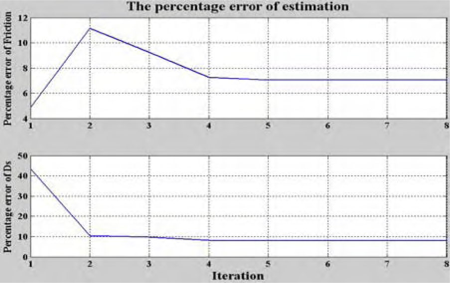
The percentage error of estimation without noise.

7. Conclusion

The experimental tests have presented the validation of estimated parameters with the experiment data from [Ngemoh97] to validate. The test results has shown that the estimated parameters can be identified up-to four parameters for this experimental tests.

Footnotes

9. Appendix

Equations for Torque Signature Signal

The mathematical model given in [1,2] is concluded below. The torque signature curve is shown by five differences stages.

Stage 1 - Screw Engagement {0 ≤ φ ≤ α}

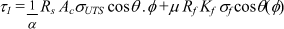
τ₁ = 1/α R_s A_c σ_UTS cos θ.φ + μ R_f K_f σ_f cosθ(φ)

Stage 2 - Screw Breaks through {α ≤ φ ≤ φ_b}

τ₂ = R_s A_c σ_UTS cos θ + 2μ R_f K_f σ_f cosθ(φ-α)

Stage 3 - Screw Full-Breakthrough {φ_b ≤ φ ≤ φ_b + α}

τ₃ = 1/α R_s A_c σ_UTS cos θ(φ_b-φ+α) + μR_fK_fσ_fcosθ(φ_b-φ-α)

Stage 4 - Screw Sliding {φ_b + α ≤ φ≤φ_t}

τ₄ = 2μR_f K_f σ_f cos θ(φ_b)

Stage 5 - Screw Tightening {φ ≥ φ_t}

τ_{5} = [(\frac{μ_{h} (D_{s h}^{3} + D_{s}^{3})}{3 (D_{s h}^{2} - D_{s}^{2})}) + (\frac{D_{s} + D_{h}}{4}) (\frac{π μ (D_{s} + D_{h}) + 2 P}{π (D_{s} + D_{h}) - 2 μ P})] [\frac{K_{t h} K_{t h}}{K_{t h} + K_{t h}}] [\frac{P (φ - φ_{t})}{2 π}]

References

Seneviratne

L.D.

Ngemoh

F.A.

and Earles

S.W.E.

(1992). “Theoretical Modeling of Screw Tightening Operations,” proceedings ASME European Joint Conference on Systems, Design and Analysis, 1992, vol. 1, pp.189–195.

Fobra.Augustine Ngemoh (1997). “Modelling the Automated Screw Insertion Process”, Ph.D. Thesis, University of London. 1997.

Visuwan

(1999). “Monitoring Strategies for Self-Tapping Screw Insertion Systems” Ph.D. Thesis, University of London, 1999.

Guzman

Bruno Lara

(2000). “Intelligent Monitoring of Screw Insertions”, Ph.D. Thesis, University of London, 2000.

Seneviratne

L.D.

Ngemoh

F.A.

Earles

S.W.E.

and Althoefer

(2001). “Theoretical modelling of the self-tapping screw fastening process”, PartC, Journal of Mechanical Engineering Science (IMechE), 215:135–154, 2001.

Klingajay

Seneviratne

L. D.

(2002). “Friction Estimation in Automated Screw Insertions”, proceedings of International Symposium on Robotics&Automation (ISRA2002), 2002, Vol.1, pp.682–688.

Klingajay

Seneviratne

L. D.

Althoefer

Kaspar

(2002), “Parameter estimation during automated screw insertions”, proceedings of 2002 IEEE International Conference on Industrial Technology (ICIT'02), 2002, Vol. II, pp.1019–1024.

Klingajay

Seneviratne

L. D.

Althoefer

Kaspar

Zweiri

Yahya H.

(2003), “Parameter Estimations for threaded assembly based on the Newton Raphson method”, proceedings of 2003 IEEE the seventh International Conference on Automation and Technology(Automation2003), 2003, Vol.1, pp. 864–869.

Klingajay

Seneviratne

L. D.

Althoefer

Kaspar

(2003). “Identification of threaded fastening parameters using the Newton Raphson Method”, proceedings of IEEE/RSJ International Conference on Intelligent Robots and Systems (IROS2003), 2003, Vol.1, pp.5055–2060.

10.

Klingajay

Seneviratne

L. D.

Giannoccaro

Nicola Ivan

(2003). “Optimization of four estimated parameters for autonomous threaded fastenings”, proceedings of 12th International Workshop on Robotics in Alpe-Adria-Danube Region, RAAD2003, 2003, Italy.

11.

Klingajay

Seneviratne

L. D.

Althoefer

Kaspar

(2004). “Model Based Automation Strategies for Threaded Assembly Systems”, proceedings of International Federation of Automatic Control (IFAC), Problems in Manufacturing (INCOM2004), 2004, Brazil.

12.

Klingajay

Giannoccaro

N. I.

(2003). “Parametric Estimation of Autonomous Threaded Fastenings Operation based on Non-linear Least Square Method”, proceedings of the ISCA 16^th International Conference: ComputerApplication in Industry and Engineering (CAINE 2003), 2003, Vol. 1, pp.211–215.

13.

Klingajay

Giannoccaro

N. I.

(2003), “Comparison between Least Square & Newton Raphson for Estimation Parameters of an Autonomous Threaded Fastenings”, proceedings of 2003 IEEE International Conference on Industrial Technology (ICIT'03), 2003, Vol. 1, pp.163–168.

14.

Fisher

R. A.

(1959). “Statistical Methods and Scientific Inference”, Oliver & Boyd, London, Second Revised Edition, Hafner Publishing Co., New York, 1959.

15.

Walsh

R. A.

(1993). “Machining and Metal working handbook,” McGraw-Hill, 1994

16.

Carl Hansen Verlag (1993). “Plastics for Engineers: Materials, Properties and Applications,”, Munich Germany, 1993

17.

Bashford

(1997). “Thermoplastics Databook,” Chapman and Hall, London, 1997.

18.

ASM V.1 (1990). “Properties and Selection: Irons, Steels and High Performance Alloys”, Metals Handbook Vol.1, ASM International, 1990.

19.

ASM V.2 (1990). “Properties and Selection: Non-ferrous alloys Special-purpose Materials”, Metals Handbook Vol.2, ASM International, 1990.

The Automated Threaded Fastening Based on On-line Identification

Abstract

Keywords

1. Introduction

2. The experimental test rig setup

2.1. Tools and manipulations

2.2 The instrument and sensor controller

2.2.1 Torque Transducer or Torque Sensor.

2.2.2 Optical Encoder

2.2.3 The reference label box or connector box

2.2.4 A Multifunction DAQ card.

3. Strategy for the on-line experimental test

3.1. Curve fitting technique on the experiment

3.2. The experiment curve identification

4. Methodology of parameter estimation

5. Analytical Model for Parameter Estimation

5. Identification of Experimental test

6. Test results

7. Conclusion

Footnotes

9. Appendix

References