Sage Journals: Discover world-class research

Abstract

In this paper, a model of visual place cells (PCs) based on precise neurobiological data is presented. The robustness of the model in real indoor and outdoor environments is tested. Results show that the interplay between neurobiological modelling and robotic experiments can promote the understanding of the neural structures and the achievement of robust robot navigation algorithms. Short Term Memory (STM), soft competition and sparse coding are important for both landmark identification and computation of PC activities. The extension of the paradigm to outdoor environments has confirmed the robustness of the vision-based model and pointed to improvements in order to further foster its performance.

Keywords

Vision hippocampus localization indoor and outdoor landmark-based navigation neural network

1. Introduction

Ethological studies of animal navigation show that a wide variety of sensory modalities can be used by the animals to navigate and to self localize. Among them, vision allows a very precise, robust and non intrusive way to navigate. Visual information can be used for taxon navigation (returning to a particular landmark) or to recognize a place from distant landmarks [Gould, 1986]. The different models of the biological vision-based navigation use the azimuth of the landmarks [Cartwright and Collett, 1983; Lambrinos 2000], more rarely, their identity or a conjunction of the two [Arleo and Gerstner, 2000; Bachelder and Waxman, 1994; Gaussier et al, 1995; Gaussier et al, 2000].

The discovery of place cells (PCs) in the rat hippocampus and also in primates has emphasized the encoding of spatial information and its use for navigation by mammalian brain [O'Keefe and Nadel, 1978; Squire, 1992]. In a first model, proposed in 1994, we showed how the learning of a few sensory-motor associations around a goal location was sufficient for a robot-like agent to exhibit a robust homing behavior [Gaussier and Zrehen, 1994] when the environment is simple (i.e. open field navigation with no need to plan a detour). A central hypothesis of our most recent model considers some aspects of hippocampal functions as devoted to the detection and fast learning of transitions between multimodal events [Gaussier et al, 2002; Banquet et al, 2005]. Hence, static PCs should exist prior the hippocampus. Model and experiments show robust PCs can be built by simple merging the what and where information coming from the visual system. We propose the merging could be performed as early as the parahippocampal region (in the perirhinal and parahippocampus cortex: PrPh). The place recognition could be performed in the entorhinal cortex (EC), the main source of input to the hippocampus and the dentate gyrus (DG), a substructure of the hippocampal system. In this view, hippocampus proper (CA1/CA3) could be devoted to the learning of transitions between places and more generally context learning. A cognitive map computes a latent learning of the spatial topology of the environment [Tolman, 1948] and can be used to plan a sequence of actions to reach an arbitrary goal [Cuperlier et al, 2005]. In this paper, we will analyse the parameters controlling the robustness of PCs in real environments. We will show that going back and forth between robotics and neurobiological modelling can help both to obtain a more robust and faster place recognition for robotics applications and explain why short term memory (STM) and soft competition mechanisms are so important for the brain functioning.

2. Model Description

This section describes a model of the prehippocampal PCs tested on different robotic platforms (Koala K-Team, Labo3 AAI, Pionner 3 AT ActivMedia), evolving in open indoor and outdoor environments. A spatial constellation of online learned landmarks (i.e. a set of triplets landmark-azimuth-elevation) defines a position in the environment and is learned by a PC. Fig. 1 summarizes the processing chain.

Fig. 1.

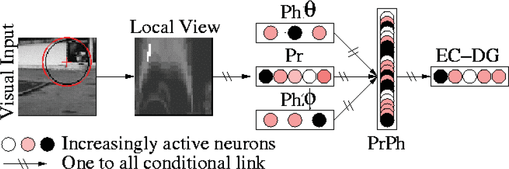
Block diagram of the architecture.

Our architecture is composed of a visual system that focuses on points of interest and extracts local views, a merging layer (PrPh) that compresses what (Pr: recognition of the current local view) and where (Ph ^θ ,Ph ^φ : azimuth and elevation) information, and a place recognition layer (EC-DG).

2.1. Landmark extraction and recognition

The first layer of the architecture is a visual system autonomously extracting landmarks from a panoramic image re-built from a set of classical image [Gaussier et al, 1997; Lepretre et al, 2000]. An omni-directional CCD camera using a conic mirror (Vstone VS-C42N-TR) has been recently introduced to speed up the experimentation [Giovannangeli et al., 2005]. This camera allows the one-shot capture of 360° panoramic images. To eliminate problems induced by luminance variability, the gradient image is the only visual input of the system (a 750×120 pixels image extracted from the 640×480 pixels panoramic image which is originally circular). The gradient image is then convolved with a DoG (Difference of Gaussian) filter to detect curvature points at a low resolution (a set of robust focus points). Finally, a log-polar transform of a small circular image centered on each focus point (which will be called a local view, somewhat different from the concept of local view in hippocampal neurophysiology) is computed in order to improve the pattern recognition when small rotations, and scale variations of the landmarks occur [Schwartz, 1980]. Fig. 2 illustrates the landmark extraction mechanism.

Fig. 2:

Illustration of landmark extraction mechanism: the gradient of a panoramic image is convolved with a DoG filter. The local maxima of the filtered image correspond to points of interest (robust focus points) which the system focuses on, to extract local views in log-polar coordinates corresponding to landmarks. The system also provides the bearing of the focus points by means of a magnetic compass. The first column represents the identity of the four most activated landmark neurons and the second column their activity level.

The recognition level L_k(t) of the current local view by the k^th neuron of Pr (i.e. the recognition level of the k^th landmark) is merely computed as a distance between the exact prototype of the k^th learned local view and the current local view:

L_{k} (t) = f^{R T} (\frac{1}{X_{I} . Y_{I}} \sum_{i, j = 1, 1}^{X_{i}, Y_{l}} ∥ ω_{i j, k}^{I = p r} (t) - 1_{i, j} (t) ∥)

with X_I and Y_iI the number of columns and rows of the local views, with $ω_{i j, k}^{I - P r} (t)$ the weight of the connection between the pixel i,j of the local view and the k^th landmark (i.e. the k^th neuron of Pr), with I_ij(t) the value of the ij^th point of the current local view, and with $f^{R T} = \frac{1}{1 - R T} [x - R T]^{+}$ an activation function that increases the dynamics of the responses.

The learning of a local view as a landmark by a new recruited neuron k of Pr occurs in one-shot according to the following learning rule (the weight is initially null):

Δ ω_{i j, k}^{I - P r} = I_{i j} (t) . R_{K}^{P r} (t)

The synapses of a Pr neuron adapt during the one-shot learning (at the recruitment, when $R_{k}^{P r} (t) = 1$ ), and do not change anymore.

In addition to a what information: the recognition of a X_I×Y_I pixels image in log-polar coordinates, the simulated visual system provides a where information: the azimuth (Ph ^θ ) and the elevation (Ph ^φ ) of the focus point (absolute direction obtained with a compass or any simulation of a vestibular system, such as a gyroscope or inertial systems). Each neuron of Ph ^θ and Ph ^φ (i.e. the neural group giving the azimuth and the elevation of the current local view) has a preferred direction and its firing rate is given by a strictly monotonous function decreasing from 1 to 0 with the angular distance between the preferred direction and the direction (θ(t), φ(t)) (azimuth and elevation) of the current extracted local view. Each neuron expresses how near the landmark is from its preferred direction.

The activity of Ph ^θ and Ph ^φ neurons is given by the following equation:

\begin{aligned} θ_{i} (t) = g^{p 1} (∥ 2. π . \frac{i}{N_{P h^{θ}}} - θ (t) ∥) \\ ϕ_{i} (t) = g^{p 2} (∥ 2. π . \frac{i}{N_{P h^{ϕ}}} - ϕ (t) ∥) \end{aligned}

with $N_{P h^{ϕ}}$ and $N_{P h^{ϕ}}$ the number of neurons in Ph ^φ and Ph ^θ , and where g^ρ(Δ _θ ) computes a lateral diffusion around the neuron which preferred direction is θ(t) (i.e. the direction of the current extracted landmark). ρ is here a parameter that defines the extent of the lateral diffusion. We propose here a simple linear diffusion but other diffusions function are possible:

g^{p} (Δ_{θ}) = {[1 - \frac{Δ_{θ}}{ρ . π}]}^{+}

with [x]⁺=x if x≥0 and 0 otherwise.

Since the visual system provides the position and the identity of the landmarks, the landmark constellation of the current place can be built.

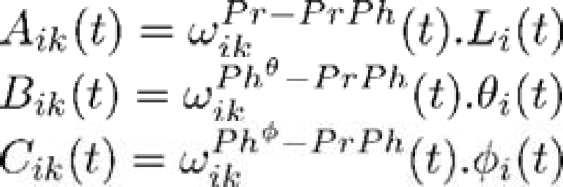
2.2 Landmark constellation building

What and where informations are merged in a product space by means of a neural third-order tensor of $N_{P r} \times N_{P h^{ϕ}} \times N_{P h^{θ}}$ neurons (with N_pr the number of neuron in the group Pr), in which each neuron is linked to a single landmark-azimuth-elevation triplet (i.e. a third-order tensor of pi-sigma units that stands in the model for the PrPh connectivity, see [Rumelhart and Zipser, 1985] for more classical sigma-pi units). A STM (short term memory) enables to remember the merging of previous inputs. At the beginning of the sequential exploration of a panorama, the STM of PrPh is reset (all the neurons are set to 0).

For each extracted local view at time t, the update of the activity of the what and where tensor M(t) (PrPh set of neuron) is given as the tensorial product of its inputs if the result is greater than the previous activity:

M (t) = max ((L \otimes θ \otimes ϕ) (t), [M (t - d t) - r (t)]^{+})

with L (resp. θ and φ) the vectorial representation of Pr (resp. Ph ^θ and Ph ^φ ), with the ⊗ operator computing a tensorial product, and with r(t) a binary tensor in which each neuron fires at the beginning of a visual exploration. The max operator between two tensors computes the tensor having for element the largest element of the two tensors. The reset of the memory of a PrPh neuron k occurs when r_k(t) fires. A biologically plausible equation of the computation of a max operator could be: max(a,b)=a+[b−a]⁺. In the following, m_k(t) is the k^th element of the tensor M. The use of the max operator is primordial since the recognition of a given landmark can occur several times during the same visual exploration (due to a mistake in the visual recognition for example). Moreover, a soft competition can be performed at the level of the landmarks recognition between neurons of Pr, allowing several interpretations of each extracted local view. Thus, the max operator has the property to select the most pertinent extracted local view since the last reset (as regard to the product between the recognition level of the local view and its spatial localisation). In the following sections, we will highlight the interest of a more sophisticated reset signal to deal with the difficulties of the focalisation system to reliably focus on learned landmarks, and the interest of a soft competition at level of the landmark recognition.

2.3 Landmark constellation building

The learning of a location triggers the learning of all the extracted landmarks based on the current panoramic image, inducing the build up of new triplets in the PrPh structure that provides a new constellation. We suppose neurons in EC-DG (i.e. the PCs) learn and recognize the activity of several PrPh units (a what and where constellation) as a pattern coding for an invariant representation of a location.

The activity of a PC results from the computation of the distance between the constellation learned by this PC and the current constellation. Thus, the activity P_k(t) of the k^th PC can be expressed as follow:

P_{k} (t) = \frac{1}{W_{k}} (\sum_{i = 1}^{N_{P r p h}} ω_{i k}^{P r P h - E C} (t) . m_{i} (t))

where $ω_{i k}^{P r P h - E C} (t) = 1$ expresses the fact that the triplet i (i.e. the i^th neuron of PrPh) whose activity is m_i(t) has been used to encode the PC k. The number of triplets used by the k^th PC is given by $W_{k} = \sum_{i = 1}^{N_{P r P h}} ω_{i k}$ with $ω_{i k} \in {0, 1}$ , and with N_PrPh the number of neurons in the what and where tensor (PrPh). The one-shot learning rule of a PC k is computed as follow (the weight is initially null):

Δ ω_{i k}^{P r P h - E C} = H_{1} (m_{i} (t)) . R_{k}^{E C} (t)

with H_y(x)=1 if x≥y and 0 otherwise (the Heaviside function). The synapses of a PC adapt during the one-shot learning (at the recruitment, when $R_{k}^{E C} (t) = 1$ ), and do not change anymore ( $R_{k}^{E C} (t) = 0$ otherwise). More precisely, the value 1 is affected to a synaptic weight if the input PrPh neurons are maximally activated (when their value is 1).

Fig. 3 proposes an experiment in which 5×5 PCs were learned at precise locations in a working room and tested in each learned and surrounded location. A remarkable property of the system relies in its built-in generalization capability: a PC coding for the location A responds when the robot is precisely in A but also to a lesser degree in the neighborhood of A, creating a continuous and large place field around A. The learning of several locations creates overlapping place fields and also leads to the paving of the space by applying a global competition. A predictable mathematical consequence of the what and where merging is the following: the shape of the place field is homothetic with the size of the environment [Gaussier et al, 2002] (i.e the shape adapts to the geometry of the environment). The prediction is verified in the experiment of the fig. 11 (large outdoor environment). On fig. 11, we can see that in an outdoor environment, the place field are really larger than in an indoor environment. In fig. 11 for instance, the place fields have a useful diameter of about 25 meters, which is almost the size of the environment. These results are coherent with the PC-like neurons recorded in the medial entorhinal cortices (in the intermediate area between the dorsal and the ventral EC) of a freely moving rat [Quirk et al, 92; Sharp, 99; Franck et al, 2000]. The system has proved to be sufficient in structured indoor environment [Gaussier et al, 1997] and has exhibited a strong robustness to environmental disturbances [Gaussier et al, 2000] when coupled with a PerAc architecture of sensori-motor navigation [Gaussier et al, 1995] based on location-action associations.

Fig. 3:

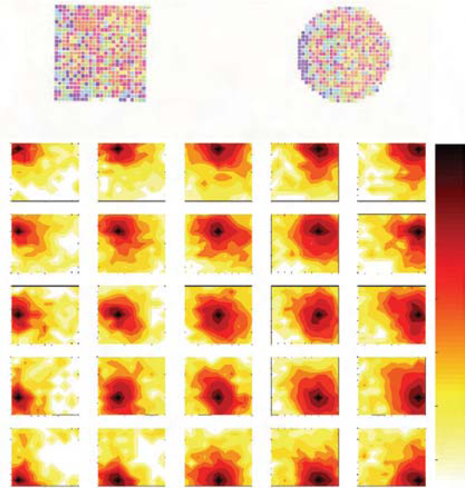
At the top, activities of neurons recorded in the entorhinal cortices of a freely moving rat in two geometrically different enclosures. At the bottom, activities of 5×5 simulated neurons recorded in a working room over about 5×6 meters (wide activity field decreasing with the distance to the learned location).

In the following, we will show that, surprisingly, the improvement of our system for dynamical indoor and outdoor environments leads to propose a more plausible model.

3. Information Compression

The use of a third-order tensor to encode what and where information is efficient but uses too many resources, and is not biologically plausible. The ratio between the number of active neurons in the PrPh tensor and the number of neurons that are really used by EC-DG is globally $\frac{N_{P r} \times \bar{n}}{N_{P r} \times N_{P h^{ϕ}} \times N_{P h}^{θ}} = \frac{\bar{n}}{N_{P h}^{ϕ} \times N_{P h}^{θ}}$ where $\bar{n}$ is the average number of different positions under which a landmark can be seen (the standard deviation of this number is σ_n). For a good precision, $N_{P h^{θ}}$ and $N_{P h^{ϕ}}$ has to be high enough (for instance 90 neurons coding for 360° in azimuth, 15 neurons coding for 60° in elevation). Thanks to generalization, the same landmark does not need to get a new code for neighboring positions. So $\bar{n}$ can be small: for example 18 different positions of a given landmark seem to be a reasonable value: 6 different azimuthal directions (angular sector of 60°) and 3 different elevations (low, average, and high). In this case, the ratio between neurons used in EC and active neurons was $\frac{18}{90.15} = \frac{1}{75}$ .

For the purpose of information compression, it is not necessary for the what and where tensor to have so many neurons. The maximum number of different positions in the visual field where a landmark can be learned (correlated to $\bar{n}$ , for example $\bar{n} + 3 σ_{n}$ ) and the number of PrPh neurons linked to one landmark (i.e. to one neuron in Pr) could be the same. But if the connectivity remains unchanged, the azimuthal precision is lost. So, in order to avoid a lost of place field precision induced by spatial discretization, each neuron of the third-order tensor PrPh can be linked to a subset of the neurons of Ph ^φ and Ph ^θ (not only a single input neuron). In this way, the same landmark will not be encoded on different spatial positions unless these positions are significantly different. This property is directly derived from the neighborhood connectivity illustrated by fig. 4.

Fig. 4:

Merging connectivity of PrPh. Each neuron is linked to one landmark neuron and a neighborhood of azimuth neurons. A single connection from this neighborhood is set to 1. The same connectivity exists at level of Ph ^φ .

Finally, a precise azimuth (resp. elevation) can be encoded by a single unitary connection between a PrPh neuron and a Ph ^θ neuron (resp. a Ph ^φ neuron). Thus, our merging tensor has a smaller number of neurons, whereas the spatial precision remains the same (90 neurons coding for 360° in azimuth, 15 neurons coding for 60° in elevation). Moreover, there is no active neuron in PrPh that has not been used by EC.

More precisely, all the connection weights are initially set to 0 downstream the PrPh tensor. The mechanism is the same: the learning of a location triggers the learning of all the extracted landmarks based on the current panoramic image, inducing the build up of new triplets in the PrPh structure defining a new constellation. The learning (or the perfect recognition) of a landmark now triggers the learning of a new triplet landmark-azimuth-elevation (i.e. the recruitment of a Pr neuron triggers the recruitment of a PrPh neuron). It is linked to the new recruited neuron in Pr and to the neurons in Ph ^θ and Ph ^φ which preferred direction is the current landmark direction. Since a single neuron of each input group Pr, Ph ^θ and Ph ^φ is maximally activated (its value is 1), the recruited PrPh neuron has a single non null (unitary) afferent synapse from each group (defining a triplet landmark-azimuth-elevation). Hence, the learning rule of a PrPh neuron j can be summarized as follow (the weight is initially null):

Δ ω_{k j}^{P r - P r P h} = H_{1} (L_{k} (t)) . R_{k}^{P r P h}

(idem with Ph ^θ and Ph ^φ instead of Pr, and θ and φ instead of L). In this equation, $ω_{k j}^{P h^{θ} - P r P h}$ (resp. $ω_{k j}^{P r - P r P h} (t)$ and $ω_{k j}^{P h^{ϕ} - P r P h} (t)$ ) is the weigth of the connection between the k^th neuron of Ph ^θ (resp. the k^th neuron of Pr and Ph ^φ ) and the j^th PrPh neuron. Hence the activity of each triplet is computed as follow:

\begin{aligned} m_{k} (t) = max (\sum_{i = 1}^{N_{P r}} A_{i k} (t) . \sum_{i = 1}^{N_{P h} θ} B_{i k} (t) . \sum_{i = 1}^{N_{P h} ϕ} C_{i k} (t) \\ , [m_{k} (t - d_{t}) - r_{k} (t)]^{+}) \end{aligned}

with

\begin{aligned} A_{i k} (t) = ω_{i k}^{P r - P r P h} (t) . L_{i} (t) \\ B_{i k} (t) = ω_{i k}^{P h θ - P r P h} (t) . θ_{i} (t) \\ C_{i k} (t) = ω_{i k}^{P h ϕ - P r P h} (t) . ϕ_{i} (t) \end{aligned}

As only one connection from Ph ^θ (resp. one connection from Ph ^φ ) has been learned, spatial precision is preserved. The compression of the information has been possible by providing a learning capability to the neurons in PrPh. Finally, unused connections are pruned after the learning, to further foster the performance (unused links downstream recruited neurons are destroyed).

This architecture, illustrated in fig. 5 is absolutely equivalent to the full third-order tensor (where the number of neurons was equal to the product of the dimensions of the three input groups). The interest of this architecture is to be faster, to use less memory, and at the same time to be more biologically plausible. The compression could be further enhanced: [Banquet et al, 2005] foresee that PrPh neurons could be linked to several perfectly distinguishable triplets of neurons landmark-azimuth-elevation from Pr, Ph ^θ and Ph ^φ (landmarks should be visually different and encoded in spatially uncorrelated place cells). Surprisingly, a more plausible model led us to a more efficient and faster system as well as trying to optimize the system has promoted the biological plausibility of the architecture.

Figure 5:

The optimized architecture: PrPh is a compact set of neuron defining a place code. Each PrPh neuron defines a triplet landmark-azimuth-elevation by means of a single unitary connection from each group.

4. Interest of Soft Competition

In this section, the interest of a more biologically plausible competition mechanism instead of a classical WTA (Winner Takes All) will be studied to deal with visual ambiguities as well as to enhance the built-in generalisation capability of the place recognition (wider place fields and place fields overlap).

A first approach to recognize a place is to suppose each local view corresponds to a single landmark. When the robot is moving from a place P_A to a place P_B, a given landmark L can be perceived as two distinct visual patterns (L₁ or L₂). Hence, in P_A, the landmark L should be recognized by the neuron L₁ and by L₂ in P_B (see Fig. 6). As shown on fig. 7, the same problem can happen even if the landmarks are on the same plane. Fig. 7 shows two landmarks N and M located on the wall of a building, learned respectively as L₁ and L₂ in place P_A, and as L₃ and L₄ in P_B. P_AP_B is 5 meters long. At the intermediate place P_C between P_A and P_B, the recognition level of each learned local view is computed. We can see L₁ and L₃ (or L₂ and L₄) have almost the same activity level and that a strict competition induces a random choice of the winner, disadvantaging one of the two PCs.

Fig. 6:

Learning using the same physical landmark seen from two different points of view. The same focus point is the center of L₁ in P_A, and L₂ in P_B. During navigation, two interpretations of the same physical landmark can compete and bias place recognition.

Fig. 7:

Learning and recognition of the same physical landmark by several neurons. The physical landmarks M and N have been learned, for two proximal locations (the two northern crosses of fig. 10, 5m distant), as different visual patterns (upper figures). Hence, in the intermediate location (place C, lower figure), the landmarks have two valid interpretations. In location C, the activity level of “L₂ and L₄” for the landmark N and the activity level of “ L₁ and L₃” for the landmark M are not displayed since they are much lower than the valid interpretations of M and N (lower than 0.82).

As the PC activity results from the product between the recognition level of what and where information (see eq. 2), allowing a single winner for the what information is equivalent to impose a maximal spatial error for all the other interpretations, even if they can be more or less valid. Choosing a single interpretation is also equivalent to consider that the landmarks corresponding to all the other interpretations are not present or not visible. Furthermore, the distance between learned prototypes shrinks with the increase in the number of encoded landmarks. Therefore, errors induced by a strict competition become more frequent (classical problem of clustering). It seems difficult and not really necessary to assign a single label to each local view. Trying to avoid the inherent ambiguity of the sensory information seems to be a mistake. Only the global behavior of the system matters [Gaussier et al, 2004; Maillard et al, 2005]. Instead of trying to perform an impossible choice, allowing multiple interpretations of the same view seems to bring a lot of advantages if the decision making (here finding the more proximal place or deciding of the current movement), is able to manage this kind of ambiguity in the code.

A solution could come from fixing a recognition threshold (RT), under which the neurons would not discharge. But it could also be difficult to optimize this parameter. Moreover, the more the system encodes landmarks, the higher the number of neurons whose activity is over this RT will be (so most of these activities will correspond to noise). Another simple solution could consist in fixing a maximum number of interpretations over a safety RT. All interpretations under this RT will be considered as wrong. If the system focuses on a novel local view, the RT should be able to inhibit a large number of neurons. In order to improve the dynamics of the landmark neurons output, the activity between RT and 1 can be linearly rescaled between 0 and 1. This is performed by the activation function f^RT(x). However, the distance between learned prototypes will decrease each time a new landmark is encoded.

So, the maximal number of valid interpretations has to be positively correlated with the number of encoded landmarks. The ratio $\frac{W}{N_{L}}$ , with W the maximal number of winning interpretations and N_L the number of encoded landmarks, must be higher than a given confidence threshold according to the landmark encoding method. Fig. 9 shows for instance the place fields induced by a strict competition, versus a soft competition. During this supervised indoor experiment, five aligned places were learned (see fig. 8). Then, the robot went over the line and PCs activity was computed at each position. Generalization expressed by place field extent and overlap is largely increased by using a soft competition. Using a strict competition prevents place fields from overlapping (see fig. 9). The sparse coding induced by soft competition allows place fields extension far from the center of the learned place, without reducing the precision in its center, as can be seen in biological EC place cells.

Fig. 8:

Room used for the experiments of the fig. 9. Crosses represent the learned positions.

Fig. 9:

Place fields induced by a strict or a soft competition (indoor env.). PC activities are computed every 2 cm over a line of 4.8 m long (see fig. 8). Places have been learned every 60 cm. Left figure shows place fields induced by a strict competition. Right figure shows place fields induced by a soft competition. A strict competition at the level of the landmark recognition does not allow a good generalization and place field overlap.

Moreover, Pr being thought to discriminate familiarity [Bogacz and Brown, 2003], a contextual computation would help to eliminate some interpretations that could not be valid in the current context computed in Pr itself. This result shows another facet of the interest of sparse coding in biological systems, instead of simple WTA. We also focused on the problem of the visual ambiguity that has to be treated since the number of learned locations (as well as the number of learned landmarks) will increase throughout the life of the robot.

5. STM in PrPh for Outdoor Environment

The functioning of the STM in PrPh can also be criticized. Indeed, in outdoor experiments, the number of visual cues and the probability to focus on the pertinent features points was much lower than in indoor environments. As a result, the outdoor experiments led to highly unstable place fields. Variability was so high that even at the position of a learned place, the PC activity could be very low (left curves of fig. 11: the same experiment as the fig. 9 was undertaken in a larger outdoor environment, see fig. 10). However, it appears that averaging activity curves or interpolating the local maximum would induce better results and help to fix the focalisation instability problem. Indeed, the analysis of the neural network during performance showed that the unstable place fields resulted from a highly variable number of learned local views the system focused on at each step. Because the images were too complex, the attention control system was unable to reliably focus on learned landmarks (low probability to retrieve them and therefore to recognize them). The question was then: could it be possible to store for a while integrated sensorial information (here the occurrences of the triplets), in order to increase the probality of using this information at each step?

Fig. 10:

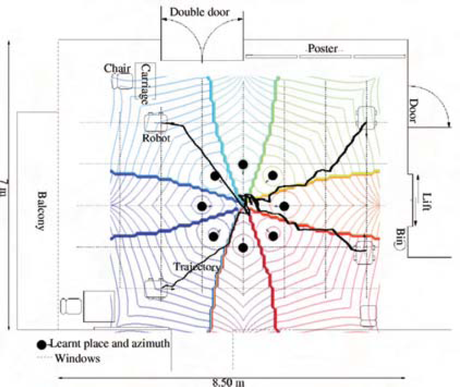
Plan of the environment used for the experiment of the fig. 11. Crosses represent the learned positions.

Fig. 11:

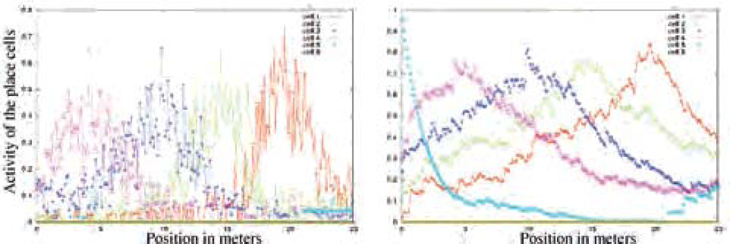
Place fields without (left) and with (right) extended STM (outdoor env.). PC activities are computed every 10 cm over a line of 25 m long (see fig. 10). Places have been learned every 5 m. Soft competition is used at the level of the landmark recognition. Left figure shows unstable place fields. Right figure illustrates the interest of a STM. In outdoor environment, the useful diameter of the place fields is about 25 m.

Obviously, mammals need not to see, step after step, every visual cue in their environment, to be able to navigate. Seeing only a few relevant cues, from time to time, seems enough to navigate without ambiguity. The existence of an extended STM at the level of the PrPh tensor would allow to remember what was seen in the previous iterations (psychological concept of working memory), and could explain why mammals do not need to verify step after step the position of each landmark. STM in the what and where tensor was previously used to store the occurrences of extracted what and where information during the exploration of the visual inputs. But the tensor was reset before the analysis of each new panorama. However, there is no need to reset so often the information of each triplet landmark-azimuth-elevation since the occurrence of a sensorial information should remain valid for a while after its integration (suppression of the global reset).

Hence, PrPh STM was increased in order to deal with the sparse or the incomplete exploration of the visual environment. We propose here for the reset signal r_k(t) of the eq. 4 the following rule:

\begin{aligned} r_{k}^{δ} (t) = [1 - H_{1} (Q_{k}^{δ} (t))]^{+} with \\ Q_{k}^{δ} (t) = m a x ([Q_{k} (t - d t) - T (t)])^{+} \\ , δ . H_{0} (m k (t) - m_{k} (t - d t))) \end{aligned}

This reset signal depends on each triplet landmark-azimuth-elevation, and occurs if the neuron has not been over-activated since a given number δ of visual explorations. T(t) is a binary signal indicating the beginning of a visual exploration of a new panorama. T(t) was previously used as the reset signal.

By means of this extended working memory, the place fields become more robust and allow a good generalization, even in outdoor environment (right curves of fig. 11).

6. Occlusion and displacement of landmarks

According to eq. 2, PC activity is a measure of the recognition of the whole learned constellation. Yet, three landmarks are mathematically sufficient to identify a position in the environment. Previous experiments have put forward the robustness of the place recognition to environmental disturbances that equally penalize all the PCs. Landmark displacements and occlusions, inducing the removal of a given number of learned landmarks, were supposed to equally penalize all the place fields. Experiments with a distorted omni-directional camera lead us to revise this assumption. Since the spatial distribution of the landmark in the different constellation can be non-uniform, an occlusion of the visual field can hide a variable number of pertinent landmarks for each cell. A more robust computation of PC activities must be introduced. As no assumption can be made about the number of pertinent landmarks in the current landmark-azimuth-elevation constellation, distance should not take into account all the learned points of the place code but rather a given ratio. This ratio must be high enough so that the computation could average the noise induced by each recognized local view (valid interpretation or not). This ratio must also be low enough to make place fields robust to the occlusions of a given number of learned landmarks. Practically, averaging the most active input terms of the sum in eq. 2 should be sufficient. PC activities are now given by the following equation:

P_{k} (t) = \frac{\sum_{m = 1}^{W_{k} . ρ_{L}} \underset{i = 1.. N_{P r P h}}{m a x^{m}} (ω_{i k}^{P r P h - E C} . m_{i} (t))}{W_{k} . ρ_{L}}

ρ_L is the ratio of pertinent landmarks necessary for the PC computation (25% of the landmarks in the following experiment because 50% of the visual field can be occluded), and ${max_{i \in I}}^{m} (x_{i})$ computing the m^th maximum in ${x_{i} \forall i \in I}$ .

In the proposed experiment of figure 12, the robot learns 5 aligned places and goes along the line formed by the places (in the same environment as in the previous outdoor experiments). During learning, a whole panoramic image is used. In order to evaluate the performance of the place recognition algorithm using this new equation, a half panoramic image is occluded after the robot has reached the intermediate position. Computation of the PC with the STM previously detailed (see eq. 4) enables the place fields to be robust to severe occlusions of the visual field and to landmark displacements. In case of such environmental disturbances, the previous computation of the PCs activity induced the place fields to collapse whereas eq. 5 enables the place field to maintain a reliable activity as long as the ρ_L % of triplet belonging to the constellation of a place cell are visible. In a spiking neuron model, it would be equivalent to consider that place cells respond as soon as the first incoming spikes.

Fig. 12:

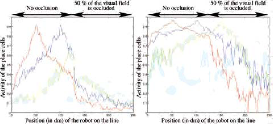
Place fields (outdoor env.) with a visual occlusion of half the panorama from the intermediate position to the and. PC activities are computed every 10 cm over a line of 25 m long (see fig. 10). Places have been learned every 5 m. Soft competition at the level of the landmark recognition, and STM previously introduced are used. Left figure shows collapsed place fields as soon as the visual field is occluded. Right figure illustrates the interest of a computation that take into account the possibility of landmark occlusion: By specifying a ratio of landmarks that has to be extracted (here, ρ_L = 25%), the PC activities do not collapse as long as this ratio of landmark can be integrated.

Modelling a visual place recognition mechanism that deals with landmark occlusions or displacements is a hard challenge. Much of the robotics algorithms only work under the assumption that the world is static at least during learning. Even if incremental SLAM (Simultaneous Localization And Mapping) methods are able to be used in real time, they are also penalized as soon as environmental changes occur. The system defined here is able to be run under the assumption that only a small part of the visual environment is pertinent, the other part being considered as unreliable. Such a property should also enable place fields to extent from a room to another room separated by an open door. This kind of robustness is also primordial in real environment where people are likely to hide a part of the visual field of the robot. Re-learning strategies are also accessible since the system is able to recognize a location that progressively changes (for example, if some objects are successively added to, or removed from the environment). Recent works have shown the interest for a robot to progressively adapt to its environment in order to navigate for a very long period in the same real and dynamic environment [Biber and Duckett, 2005]. Our model of pre-hippocampal PC allows a homing behavior and generalization of the sensory-motor learning over a very important distance (see fig 1). Moreover, our PCs do not correspond to the features of PCs found in the hippocampus proper (CA1/CA3 region), but rather to the characteristics of entorhinal or subicular PC [Quirk et al, 92; Sharp, 99; Franck et al, 2000]. Our results confirm that simple navigation tasks could be performed by broad prehippocampal PCs, and that hippocampal PCs could be built from a strong competition between these cells (in our model, CA3/CA1 neurons predict transitions between the current place and the next possible places).

7. Conclusion

In this paper, it was shown that the interaction between robotics and neurobiology leads to introduce more biological plausibility in our model, to increase the performance and the robustness of the system, and to explain the importance of STM and soft competition in brain functioning. Experiments of sensori-motor navigation, using the PCs architecture proposed here, have also been successfully achieved in indoor environment. Fig. 13 summarizes the sensori-motor mechanism based on associations between places and movement around a goal. Generated trajectories as well as the theoretical attraction basin are superimposed on fig. 14. The system has been intensively evaluated in indoor environment, and exhibits a really strong robustness to dynamical aspects of the real environment (moving people, luminance changing, landmark removal and addition, obstacle avoidance…). Outdoor experiments have also highlight the interest of a more sophisticated attentional system, that would help identifying and retrieving more robust landmarks.

Fig. 13:

Principle of the sensory-motor homing behaviour in indoor environment. The robot learns a given number of locations around a goal and associates the movement to execute in order to come back to the goal.

Fig. 14:

Real trajectories of homing in indoor environment. 8 places (black circles) are learnt at 1 m from the goal (size of the square of the floor). The theoretical place fields are superposed with the plan and the trajectories. The behavior of the robot is coherent with the theoretical attraction basin.

In future models, other visual cues such as distance deduced from parallax effects, color and textures information, will be taken into account for a better characterization of the landmarks.

In future works, navigation experiments should be undertaken in large outdoor environments (more than 1 km.).

Our results also suggest that, even in outdoor environment, no Cartesian map information is necessary for a robust navigation. However, as visual information is sometime limited, iodiothetic information could help to disambiguate the recognition of complex dynamic environments, and allothetic information could help maintaining a coherent idiothetic space representation [Arleo and Gerstner, 2000; Redish and Touretzky, 1997]. But we claim, as opposed to other models of hippocampal function [McNaughton et al, 1996], that visual information is preponderant. Outdoor and indoor navigation has always been studied separetely by most of the robotician [DeSouza and Kak, 2002].

SLAM methods offer efficient systems for closed indoor and structured environment [Thrun, 2002] and impressive robustness when coupled with vision-based localisation that enables to deal with the correspondence problem [Andreasson et al, 2005], but these technics would encounter accuracy problems when confronted to less structured outdoor environments. Outdoor navigation is a more broad problem covering rough terrain exploration [Chatilla, 1995], GPS based navigation (DARPA Challenge), cartesian elevation map for safe navigation in rough terrain, safe unmanned vehicle guidance in urban environment [Royer et al, 2005], road or path following. All these applications are really different from the concern of indoor navigation. For a long time, the field of biomimetic navigation has been considered as marginal from the robotic view point, but offers a relevant issue to reconcile outdoor and indoor navigation as illustrated by our work and a few others [Prasser et al, 2005].

Since the different biomimetics modelizations are segregated by the cognitive complexity of the task and not by the field of application [Franz and Mallot, 2000], this field of the robotics on one hand provides an essential evaluation platform for neurobiological and psychological model and on the other hand offers a different yet pertinent approach to robotic system design. Videos are available on: http://www.etis.ensea.fr/∼neurocyber/Videos/homing/index.html

Footnotes

Appendix

Pano. is the size of the panoramic image. Deriche is the classical parameter A of a Deriche gradient computation used in the experiments. Dog. σ₁, Dog σ₂> and Dog size define the DoG filtering window used to extract the focus points. Radius is the radius in pixels of the extent of the log-polar transformation (radius of the circles on fig. 2). Nb. Int. is the number of allowed interpretations in the computation process between the landmark neurons. The other parameters are defined in the paper.

Acknowledgments

These researches are supported by the Delegation Generale pour l'Armement (DGA), project no 04 51 022 00 470 27 75. We particularly thank G. Desilles for his useful collaboration. The Institut Universitaire de France also contributes to our studies.

References

[ Andreasson , 2005] Andreasson

Treptow

and Duckett

. Localization for Mobile Robots using Panoramic Vision, Local Features and Particle Filter. In IEEE International Conference on Robotics and Automation (ICRA 2005), Barcelona, Spain, 18–22, 2005.

[ Arleo and Gerstner , 2000] Arleo

and Gerstner

. Spatial cognition and neuro-mimetic navigation: A model of hippocampal place cell activity. Biol. Cybern., 83(3):287–299, 2000.

[ Bachelder and Waxman , 1994] Bachelder

I. A.

and Waxman

A. M.

. Mobile robot visual mapping and localization: A view-based neurocomputational architecture that emulates hippocampal place learning. Neural Networks, 7(6/7):1083–1099, 1994.

[ Banquet , 2005] Banquet

J. P.

Gaussier

Quoy

Revel

, and Burnod

. A hierarchy of association in hippocampo-cortical systems: cognitive maps and navigation strategies. Neural Computation, 17:1339–1384, 2005.

[ Biber and Duckett , 2005] Biber

and Ducket

. Dynamic Maps for Long-Term Operation of Mobile Service Robots. In Proceedings of Robotics: Science and Systems I, Cambridge, MA, USA, 2005.

[ Bogacz and Brown , 2003] Bogacz

and Brown

M. W.

. Comparison of computational models of familiarity discrimination in the perirhinal cortex. Hippocampus, 13:494–524, 2003.

[ Cartwright and Collett , 1983] Cartwright

B. A.

and Collett

T. S.

. Landmark learning in bees. Journal Comp. Physiology, 151:521–543, 1983.

[ Chatilla , 1995] Chatilla

. Deliberation and reactivity in autonomous mobile robots. Robotics and Autonomous Systems, 16(2-4):197–211, December 1995.

[ Cuperlier , 2005] Cuperlier

Quoy

Gaussier

and Giovannangeli

. Navigation and planning in an unknown environment using vision and a cognitive map. In IJCAI-05 Workshop: Reasoning with Uncertainty in Robotics (RUR-05), 2005.

10.

[ DeSouza and Kak , 2002] DeSouza

G. N.

and Kak

A. C.

. Vision for mobile robot: a survey. IEEE Trans. on Pattern Analysis and Machine Intelligence, 24(2):237–267, 2002.

11.

[ Franck , 2000] Franck

Brown

, and Wilson

. Trajectory encoding in the hippocampus and entorhinal cortex. Neuron, 27:169–178, 2000.

12.

[ Franz and Mallot , 2000] Franz

M. O.

and Mallot

H. A.

. Biomimetic robot navigation. Robotics and Autonomous System, 30:133–153, 2000.

13.

[ Gaussier and Zrehen , 1994] Gaussier

and Zrehen

. Navigating with animal brain: a neural network for landmark identification and navigation. In Proceedings of Intelligent Vehicles. Paris IEEE Press, 1994.

14.

[ Gaussier and Zrehen , 1995] Gaussier

and Zrehen

. PerAc: A Neural Architecture to Control Artificial Animals. Robotics and Autonomous System, 16(2-4):291–320, 1995.

15.

[ Gaussier , 1997] Gaussier

Joulain

Zrehen

Banquet

J. P.

, and Revel

. Visual navigation in an open environment without map. In International Conference on Intelligent Robots and Systems - IROS'97, pages 545–550, Grenoble, France, September 1997. IEEE/RSJ.

16.

[ Gaussier , 2000] Gaussier

Joulain

Banquet

J. P.

Lepretre

, and Revel

. The visual homing problem: an example of robotics/biology cross fertilization. Robotics and autonomous system, 30:155–180, 2000.

17.

[ Gaussier , 2002] Gaussier

Revel

Banquet

J. P.

, and Babeau

. From view cells and place cells to cognitive map learning: processing stages of the hippocampal system. Biological Cybernetics, 86:15–28, 2002.

18.

[ Gaussier , 2004] Gaussier

Baccon

J. C.

Prepin

Nadel

, and Hafemeister

. Formalization of recognition, affordances and learning in isolated or interacting animats. In From Animals to Animats: SAB'04, pages 57–66, Cambridge, MA, MIT Press, 2004.

19.

[ Giovannangeli , 2005] Giovannangeli

Gaussier

and Banquet

. Robot as a tool to study the robustness of visual place cells. In I3M'2005: International Conference on Conceptual Modeling and Simulation (CMS 2005), pages 97–104, Cambridge, Marseille, 2005.

20.

[ Gould , 1986] Gould

J. L.

. The biology of learning. Annual Review of Psychology, 37:163–192, 1986.

21.

[ Lambrinos , 2000] Lambrinos

Moller

Labhart

Pfeifer

Wehner

. A mobile robot employing insect strategies for navigation, Robotics and Autonomous Systems, 30:39–64, 2000.

22.

[ Lepretre , 2000] Leprêtre

and Gaussier

and Cocquerez

J. P.

From Navigation to Active Object Recognition The Sixth International Conference on Simulation for Adaptive Behavior SAB'2000, MIT Press, 266–275, 2000.

23.

[ McNaughton , 1996] McNaughton

B. L.

Barnes

C. A.

Gerrard

Gothard

Jung

Knierim

Kudrimoti

Qin

Skagges

Suster

, and Weaver

. Deciphering the hippocampal polyglot: the hippocampus as a path integration system. Journal of Experimental Biology, 119:173–185, 1996.

24.

[ Maillard , 2005] Maillard

Gapenne

Hafemeister

, and Gaussier

. Perception as a dynamical sensori-motor attraction basin. In Advances in Artificial Life (8th European Conference, ECAL), Springer-Verlag, 37–46, 2005.

25.

[ O'Keefe and Nadel , 1978] O'Keefe

and Nadel

. The hippocampus as a cognitive map. Clarendon Press, Oxford, 1978.

26.

[ Prasser , 2005] Prasser

Milford

M. J.

Wyeth

. Outdoor Simultaneous Localisation and Mapping using RatSLAM In International Conference on Field and Service Robots, Port Douglas, Australia, 2005.

27.

[ Quirk , 1992] Quirk

G. J.

Muller

R. U.

Kubie

J. L.

and Ranck

J. B.

Jr. The positional firing properties of medial entorhinal neurons: Description and comparison with hippocampal place cells. Journal of Neuroscience, 12(5):1945–1963, 1992.

28.

[ Redish and Touretzky , 1997] Redish

A. D.

and Touretzky

D. S.

. Cognitive maps beyond the hippocampus. Hippocampus, 7(1):15–35, 1997.

29.

[ Royer , 2005] Royer

Bom

Dhome

Thillot

and Marmoiton

. Outdoor autonomous navigation using monocular vision. In IEEE/RSJ IROS2005 International Conference on Intelligent Robots and Systems, 3395–3400.

30.

[ Rumelhart and Zipser , 1985] Rumelhart

D. E.

and Zipser

. Feature discovery by competitive learning. Cognitive Science, 9:75–112, 1985.

31.

[ Schwartz , 1980] Schwartz

. Computational anatomy and functional architecture of striate cortex: a spatial mapping approach to perceptual coding. Vision Res., 20:645–669, 1980.

32.

[ Sharp , 1999] Sharp

. Complementary roles for hippocampal versus subicular/entorhinal place cells in coding place, context, and events. Hippocampus, 9(4):432–443, 1999.

33.

[ Squire , 1992] Squire

L. R.

. Memory and the hippocampus: A synthesis from findings with rats, monkeys, and humans. Psychological Review, 99:143–145, 1992.

34.

[ Tolman , 1948] Tolman

E. C.

. Cognitive maps in rats and men The Psychological Review, 55:189–208, 1948.

35.

[ Thrun , 2002] Thrun

. Robotic Mapping: A Survey. In Exploring Artificial Intelligence in the New Millenium. Lakemeyer

and Nebel

, eds. Morgan Kaufmann, 2002.

Robustness of Visual Place Cells in Dynamic Indoor and Outdoor Environment

Abstract

Keywords

1. Introduction

2. Model Description

2.3 Landmark constellation building

Footnotes

Appendix

Acknowledgments

References