Sage Journals: Discover world-class research

Abstract

Nowadays the size and dimension of mobile manipulators have been decreased for being usable in various regions. This leads several problems such as danger of instability. Therefore, many researches have been done to overcome the problem of overturning of a mobile manipulator. In this paper, an algorithm for increasing the stability of a mobile manipulator is presented based on the optimization of a performance index. The path of vehicle and the desired task of the end-effector are predefined. In order to apply the optimal stability criterion, it is more convenient that the manipulator be of a redundant. Considering the interaction between the vehicle and the manipulator and using the genetic algorithm to minimize the stability criterion cooperating with a neural network, the proposed method is a swift algorithm to determine the optimum configuration of the manipulator for real time overturning control of the vehicle. An example for illustrating the significance of the proposed method is presented in a two dimensional configuration.

Keywords

Mobile manipulator redundant optimal stability Real-Time control neural network

Nomenclature

a_x, a_y, a_z

Acceleration of center of mass of vehicle in the direction of principle axes

f_x, f_y, f_z

Reaction forces from manipulator acting on the vehicle

M_x, M_y, M_z

Moments from manipulator acting on the vehicle

F_{X_{w i}}, F_{Y_{w i}}, F_{Z_{w i}}

Road reaction on the tire i

X̂_i, Ŷ_i, Ẑ_i

Principal directions

P_x, P_y, P_z

Position of end-effector in the principal directions

L_i

Length of link i

m_i

Mass of link i

Mass of vehicle

Distance between Ẑ₀ and Ẑ₁ in X̂₀ direction

Angle between tangent to the path of end-effector and the horizon

Distance of end-effector from origin in direction Ŷ₀

Velocity of vehicle

v′

Velocity of end-effector

θ _i

Angle between X̂_i-1 and X̂_i around Ẑ_i

{\dot{θ}}_{i} = ω_{i}

Angular velocity of link i

{\ddot{θ}}_{i} = α_{i}

Angular acceleration of link i

ⁱ ω^j

Angular velocity of link j expressed in frame {i}

ⁱ ω̇^j

Angular acceleration of link j expressed in frame {i}

ⁱP_j

Position vector located at the end point of link j expressed in frame {i}

^{i} P_{C_{j}}

Position vector located at the mass center of link j expressed in frame {i}

ⁱv̇_j

Acceleration of origin of frame {j} expressed in frame {i}

^{i} {\dot{v}}_{C_{j}}

Acceleration of mass center of link j expressed in frame {i}

ⁱN_j

Moment acting on mass center of link j by link j − 1 expressed in frame {i}

ⁱn_j

Moment acting on link j by link j − 1 expressed in frame {i}

ⁱF_j

Force acting on mass center of link j by link j − 1 expressed in frame {i}

ⁱf_j

Force acting on link j by link j − 1 expressed in frame {i}

τ_i

Torque acting on link i by link i − 1

^{C_{i}} I_{i}

Central inertia tensor for link i

ⁱẐ_i

Unit vector in Z direction

_jⁱR

Rotation matrix of arm j expressed in frame {i}

1. Introduction

A significant problem in the field of automated mobile manipulators is the issue of stability. A mobile manipulator is a multi-link arm with ability to move in a plane or space which is mounted on a vehicle. Current applications of mobile manipulators in unknown environments such as planet exploration have been done on small-sized mobile manipulators [1, 2, and 3]. These systems may have especial and important tasks such that these missions can result instability leading to overturning. Although the motion of manipulator may have universe effects on the stability of the card, because of dynamic interface between the vehicle and manipulator, the action of manipulator may be controlled to compensate the threshold of stability.

In addition to the stability, there are some other important factors that may be considered in analyzing a moving robot. These tasks minimize the time of motion or minimize the consuming energy of a moving robot system along its motion. For optimizing these subjects in a mobile manipulator, one way is that the manipulator be of a redundant type. Having redundancy in a robot system, the order of complexity of dynamical equations significantly increases. Nonetheless, it has been shown although this intricacy of dynamic equations may cause us troubles, it is possible to easily conquer the instability of the mobile manipulator.

Huang et al. have done various researches on mobile manipulators [4, 5, and 6]. In [4] manipulator motion planning for stabilizing a mobile manipulator has been considered. They have derived the cooperative motions of the vehicle and the manipulator for a stabilization which is compatible with task operation so the mobile manipulator can successfully accomplish tasks in environments with various disturbances. The authors used a method based on Zero Moment Point (ZMP) for their study.

A method for coordinating vehicle motion planning is presented in [5]. This study considers manipulator task constraints and manipulator motion planning considering platform stability. The method of ZMP path planning by a stability potential field is presented in [6]. Based on this method, a motion planning algorithm is formulated to control the manipulator in order to maintain the stability of the whole system while the vehicle is moving along a given trajectory.

An efficient algorithm for controlling the angular momentum of walking robots through the manipulation of the Zero Moment Point (ZMP) is presented by Mitobi and et al. [7]. A remarkable feature of their control method is that the ZMP is considered an actuating signal of the controller. The proposed method can be applied in real time situations because it does not need an accurate tracking of joint angles.

Dynamic motion planning of autonomous vehicles is presented by Shiller et al. [8]. A method for planning the motion of autonomous vehicles moving on general terrains has been presented. The kinematics of the vehicle for its orientation and steering angle along the path is derived. Next vehicle dynamics are derived in terms of path geometry, and the constraints on vehicle motions are formulated in this paper. Further the terrain and the path representations and also local and global optimizations are briefly discussed in the last part.

Tipover stability estimation for autonomous mobile manipulators using neural network has been considered by Meghdari et al. [9]. The proposed approach is a neural network based algorithm that is capable of detecting an instable situation in a mobile manipulator and is fast enough to prevent tipover.

Increasing stability of mobile manipulator using dynamic compensation has been studied by Meghdari et al. [10]. The stability of a mobile manipulator has a close relation with the vehicle's motion. A redundant manipulator provides a better performance on a mobile manipulator which is to move and perform a predefined task. By using this redundancy and applying the optimal parameters, they have increased the stability of mobile manipulator. The genetic algorithm is frequently used as an alternative optimization tool to conventional methods for training and adaptation of parameters in dynamical systems. In many cases, the GA technique is integrated in neural networks as the component of the hybrid optimization approach [11].

In this paper, the nonlinear equations of a mobile manipulator which moves in a vertical plane have been derived. The measure for determining the stability criterion of the mobile manipulator is the tires upward force [9]. By having this measure, first, for real-time control with dynamic compensation motion of manipulator, a neural network database has been trained for the solutions of the nonlinear equations. This neural network cooperates with genetic algorithm in order to minimize a performance index according to the optimal stability. Afterwards, a PD controller controls the angular position and angular velocity of each joint such that the error and the derivation of error becomes zero.

2. The Dynamic Model of a Mobile Manipulator

In this section, a three degrees-of-freedom manipulator with ability to move in a vertical plane which is mounted on a 4-wheeled vehicle is considered. The Newton's law is employed in deriving the dynamic equation in this paper. Because of the especial task of the mobile manipulator, the path of vehicle and the desired task of the end-effector are predefined. Thus there are some limited configurations of manipulator while moving along its desired path. These arrangements of manipulator do not satisfy the stability criterion when the upward force of each tire tends to zero. To solve this problem, one way is that the manipulator be of a redundant type.

The schematic picture of a redundant 3 degrees-of-freedom manipulator with attached coordinates to its links is shown in Fig. 1. The free body diagram of the vehicle is also shown in this figure.

Fig. 1.

Schematic diagram of a 3 degrees-of-freedom manipulator with free body diagram of the vehicle

By using the Denavit-Hartenberg notation [12], it is feasible to find the kinematic equations of the mobile manipulator. The Denavit-Hartenberg parameters and variables are shown in Table 1. It is assumed that the system is at the steady state condition where its vehicle velocity is constant.

Table 1.

Denavit-Hartenberg parameters and variables

i	α_{i − 1}	θ_{i − 1}
1	a	0
2	0	θ₁
3	L ₁	θ₂
4	L ₂	θ₃
5	L ₃	0

In Table 1, the first row relates the inertial coordinate to the body coordinate attached to the common point of the manipulator and vehicle (this row is optional). The fifth row is a pure translation that transforms the frame 4 to the frame 5.

The forces and torques equations in x-y plane are as follows:

F_{y 1} + F_{y 2} + F_{y 3} + F_{y 4} + f_{y} - M g = m a_{y}

(1)

\begin{aligned} b (F_{y 2} + F_{y 4}) + (- M g + f_{y} + m a_{y}) \frac{b}{2} - h f_{x} \\ + M_{z} - \frac{h}{2} m a_{x} = 0 \end{aligned}

(2)

Assuming that the vehicle of mobile manipulator is symmetric with respect to x-y plane, it is clear that the forces F_y1 and F_y3 are equal and also F_y2 is equal to F_y4. Considering the vehicle at the steady state conditions, where velocities at different directions are constant, we have:

a_{x} = a_{y} = a_{z} = 0

(3)

The kinematic equations may be found by using the Denavit-Hartenberg parameters from Table 1 and the general transformation matrices:

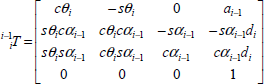
_{i}^{i - 1} T = [\begin{matrix} c θ_{i} & - s θ_{i} & 0 & a_{i - 1} \\ s θ_{i} c α_{i - 1} & c θ_{i} c α_{i - 1} & - s α_{i - 1} & - s α_{i - 1} d_{i} \\ s θ_{i} s α_{i - 1} & c θ_{i} s α_{i - 1} & c α_{i - 1} & c α_{i - 1} d_{i} \\ 0 & 0 & 0 & 1 \end{matrix}]

(4)

Where, expressions ‘c’ and ‘s’ denote the cosine and sine of the angle, respectively.

By multiplying sequentially the transformation matrices from the initial frame to the end-effector frame, the kinematic equations may be found as follows:

P_{x} = a + L_{1} \cos (θ_{1}) + L_{2} \cos (θ_{1} + θ_{2}) + L_{3} \cos (θ_{1} + θ_{2} + θ_{3})

(5)

P_{y} = L_{1} \sin (θ_{1}) + L_{2} \sin (θ_{1} + θ_{2}) + L_{3} \sin (θ_{1} + θ_{2} + θ_{3})

(6)

The velocities and acceleration equations of the end-effector can also be determined by differentiating from equations (5) and (6) with respect to time.

Therefore, for solving the inverse kinematics of the system, two equations for the position of the end-effector in the x-y plane, two equations for velocity of the end-effector are employed. These are further to the two equations for the acceleration of the end-effector which are zero in this work. The 9 unknown variables are; θ₁, θ₂, θ₃ for angular positions, ${\dot{θ}}_{1}, {\dot{θ}}_{2}, {\dot{θ}}_{3}$ for angular velocities and ${\ddot{θ}}_{1}, {\ddot{θ}}_{2}, {\ddot{θ}}_{3}$ , for angular accelerations, respectively. Subsequently, the method for determining the 9 unknown variables with 6 equations will be discussed.

For optimal stability of the mobile manipulator, the summation of tires upward forces F_y1, F_y3 should be set equal to the summation of forces F_y2 and F_y4. This leads us to define a performance index to be at its minimum value during the motion of mobile manipulator.

This performance index can be set equal to the torque exerted on the first joint of manipulator attached to the vehicle. This equation is calculated by Lagrangian method and its accuracy is checked with the Newton-Euler iteration technique [13]. The general form of the external and internal iterative relations is given in appendix 1. The torque acting on the first joint attached to the vehicle is as follow:

\begin{aligned} τ_{1} = m_{1} {L^{2}}_{1} {\ddot{θ}}_{1} + m_{2} {L^{2}}_{1} {\ddot{θ}}_{1} + m_{2} {L^{2}}_{2} ({\ddot{θ}}_{1} + {\ddot{θ}}_{2}) + 2 m_{2} L_{1} L_{2} c_{2} {\ddot{θ}}_{1} + m_{2} L_{1} L_{2} c_{2} {\ddot{θ}}_{2} + \\ m_{3} {L^{2}}_{1} {\ddot{θ}}_{1} + m_{3} {L^{2}}_{2} ({\ddot{θ}}_{1} + {\ddot{θ}}_{2}) + m_{3} {L^{2}}_{3} ({\ddot{θ}}_{1} + {\ddot{θ}}_{2} + {\ddot{θ}}_{3}) + 2 m_{3} L_{1} L_{2} c_{2} {\ddot{θ}}_{1} + m_{3} L_{1} L_{2} \\ c_{2} {\ddot{θ}}_{2} + 2 m_{3} L_{1} L_{3} c_{23} {\ddot{θ}}_{1} + m_{3} L_{1} L_{3} c_{23} {\ddot{θ}}_{2} + m_{3} L_{1} L_{2} c_{23} {\ddot{θ}}_{3} + 2 m_{3} L_{2} L_{3} c_{3} {\ddot{θ}}_{1} + 2 m_{3} L_{2} \\ L_{3} c_{3} {\ddot{θ}}_{2} + m_{3} L_{2} L_{3} c_{3} {\ddot{θ}}_{3} - 2 m_{3} L_{1} L_{2} s_{2} {\dot{θ}}_{1} {\dot{θ}}_{2} - m_{3} L_{1} L_{2} s_{2} {\dot{θ}}_{1}^{2} - 2 m_{3} L_{1} L_{3} s_{23} {\dot{θ}}_{1} ({\dot{θ}}_{2} + \\ {\dot{θ}}_{3}) - m_{3} L_{1} L_{3} s_{23} {\dot{θ}}_{2} ({\dot{θ}}_{2} + {\dot{θ}}_{3}) - m_{3} L_{1} L_{3} s_{23} {\dot{θ}}_{3} ({\dot{θ}}_{2} + {\dot{θ}}_{3}) - 2 m_{3} L_{2} L_{3} s_{3} {\dot{θ}}_{1} {\dot{θ}}_{3} - 2 \\ m_{3} L_{2} L_{3} s_{3} {\dot{θ}}_{2} {\dot{θ}}_{3} - m_{3} L_{2} L_{3} s_{3} {\dot{θ}}_{3}^{2} + m_{1} g L_{1} c_{1} + m_{2} g L_{1} c_{1} + m_{2} g L_{2} c_{12} + m_{3} g L_{2} c_{12} \\ + m_{3} g L_{2} c_{12} + m_{3} g L_{3} c_{123} - 2 m_{2} L_{1} L_{2} s_{2} {\dot{θ}}_{1} {\dot{θ}}_{2} - m_{2} L_{1} L_{2} s_{2} {\dot{θ}}_{2}^{2} \end{aligned}

(7)

3. Neural Network Theory

In general, a neural network is a system with a parallel connection among its elements which is able to model the extremely complex systems. In this case a chain of inputs consequences outputs. This kind of network can predict new observations by detecting the past observations. Neuron is the smallest unit of processing information which is the basis of neural network performance. Neural networks are generally composed of some layers. These layers are created from a number of internally connected nodes which hold an activation function. Models are presented to the network by means of the input layer, which communicates to one or more hidden layers in which the real processing is done via a system of weighted connections.

The hidden layers then are connected to the output layer as illustrated in Fig. 2.

Fig. 2.

An example of a neural network structure with 3 layers

There are some methods for training but one of them is the perceptron algorithm that we can show it by the following steps [14]:

Initiating the weighting functions and thresholds arbitrarily

Giving an input to the network

Calculating the outputs by comparing the summation of weighting functions and threshold

Diminishing the error by modifying the weighting functions

Giving the further input to the model …

For a multi-layer perceptron algorithm we use the following relation:

w_{i j} (t + 1) = α w_{i j} (t) + η δ_{p j} o_{p j}

(8)

Where, α is momentum, w_ij represents the weighting function from node i to node j at time t, η is learning rate, δ_pj relates the error term corresponding to the p pattern in node j, o_pj is the output of node j corresponding to the p pattern.

The optimum values of η and α are calculated such that the predictor error be minimized.

Standard backpropagation is a gradient descent algorithm where the network weights are moved along the negative of the gradient of the performance function. The term backpropagation refers to the method in which the gradient is calculated backward for nonlinear multilayer networks.

Usually, a new input will lead to an output similar to the correct output for input vectors used in training that are similar to the new input being presented. This generalization property makes it possible to train a network on a representative set of input/target pairs. Then it gets good results without training the network on all possible input/output pairs [15].

4. Numerical Example and Simulation Results

In Fig. 3 the picture of a 3 degrees-of-freedom manipulator mounted on a vehicle is illustrated. The manipulator is of a redundant type with the purpose of creation an infinite number of configurations for manipulator such that the end-effector be bale to track a desired path. At this case, there is a configuration that can minimize a performance index, as a measure for optimal stability criterion. Because of especial mission of the mobile manipulator, the paths of the end-effector and vehicle are predefined. In Fig. 3, it is assumed that the manipulator moves in a vertical plane and both the manipulator and the vehicle are moving with a constant velocity.

Fig. 3.

A 3 degrees-of-freedom manipulator mounted on a vehicle which moves with a constant velocity

By applying genetic algorithm, it is assumed that the quantities $θ_{1}, {\dot{θ}}_{1}, {\ddot{θ}}_{1}$ are as inputs and the performance index which is the difference between the tires upward force be as output. For this purpose, the GA toolbox of MATLAB has been used.

Noting that the first joint of the manipulator is the joint attached to the vehicle, then the performance index J, is defined as the absolute value of the torque M_z or τ₁ acting on the first joint in the z direction:

J = | M_{z} |

(9)

The value of J in (9) is equal to the torque τ₁ in equation (7). This torque directly affects the upward forces of tires. The minimum value of J depends on the geometry of the total system. In this case, when the center of mass is located at the same vertical direction as the first joint attached to the vehicle, then the four upward forces of tires are identical. In other words, the difference between the upward force of rear tires should be set equal to the upward force of the frontier tires.

The required time for calculating the performance index is so much that it causes this method to be unfeasible. In order to derive the best configuration for the mobile manipulator in the shortest time, a neural network has been applied. This network helps one for real-time compensatory manipulator motion for stabilizing the mobile manipulator.

For creating a database, first it should be determined that which parameters vary and how much is their variation range. Then the dynamic equations are solved by varying the related parameters such that a neural network database will be created. This database covers a large number of cases that may happen in the system. By using this database, the neural network will be able to find the best configuration of the manipulator which minimizes the performance index very swiftly. A PD controller is used to create the appropriate torque to be exerted on each joint of the manipulator. Thus control law must direct the manipulator to the certain path. Regarding the dynamical effects, the coefficient of PD controller can be found. Also parameters which vary and their variation range are given in Table 2.

Table 2.

Variable increment for training

Variables	Variation Range	Increment
v(m / s)	0.5 – 1.4	0.15
α (rad)	0.1 – 1.1	0.2
b(m)	0 – 0.6	0.1
P_y(m)	0 – 2.1	0.3

Table 2 shows the velocity v of the vehicle, angle α, vertical distance b, and vertical position of the end-effector P_y respectively. The database is composed of 2352 data. These four variables cover the entire cases which may happen for the mobile manipulator while moving.

Every datum is made up of four inputs, as given in Table 2, and three outputs $θ_{1}, {\dot{θ}}_{1}, {\ddot{θ}}_{1}$ . These values are calculated to minimize the performance index.

For training process, the Tevenberg-Marquardt (TM) algorithm with neural network toolbox of MATLAB are used. The specifications of the neural network are given in Table 3.

Table 3.

Specifications of the trained neural network

Network Type	Feed-Forward Back-Propagation
Adaptation learning function	Gradient Descent with Momentum (learngdm)
Performance function	Mean Square Error (MSE)
Number of Layers	3
Layer 1	25 neurons, Transfer function: Tansig
Layer 2	20 neurons, Transfer function: Tansig
Layer 3	3 neurons, Transfer function: Purelin
Epochs	800

Hidden and output layer weights are shown in Table 4.

Table 4.

Weights of different layers

Weights of hidden layer 1	Weights of hidden layer 2	Weights of output layer
8.2391	0.054365	0.83439
82.9405	−0.1651	−0.98739
8.3698	−0.46296	−0.028441
0.20165	−0.20858	–
104.4925	0.32039	–
0.22286	−0.63339	–
−4.0778	−0.85822	–
−1.234	−0.41555	–
−10.5341	0.34458	–
0.75839	0.23502	–
−24.2129	−0.56573	–
8.2239	−0.16548	–
−49.7908	−0.4395	–
−55.8598	−0.98928	–
−2.0596	−0.39226	–
−3.6826	−0.42803	–
1.2304	−0.18805	–
−28.9436	0.083442	–
0.41686	0.3358	–
−37.4119	0.15397	–
60.7128	–	–
32.1877	–	–
107.7949	–	–
−4.7371	–	–
−34.7591	–	–

The effectiveness of the learned neural network is shown in Fig. 4. This diagram is extracted for 50 sample points from the lookup table. The accuracy of the neural network is tested by comparing the data directly obtained from the appropriate equations and obtained from the learned neural network.

Fig. 4.

50 Sample points for θ₁

Since the neural network has been implemented, by referring to the database, the appropriate values can be accessed for optimal stability and it is possible to control the system On-line.

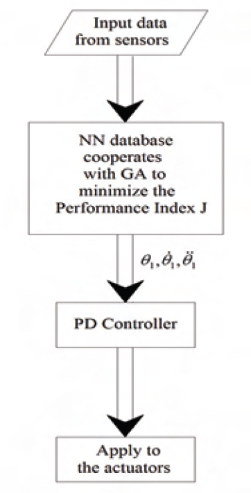
The structure for the proposed algorithm is illustrated in Fig. 5. As shown in this figure, input data is, first, obtained from sensors. Then these inputs activate the neural network unit which cooperates with an internally genetic algorithm in order to create a database and minimize the performance index. Then the outputs of neural network block enter a control block and determine the required torque that must be exerted on each joint for making the optimum configuration of manipulator. Finally, these values will be sent as an electrical or voltage signal to the actuators.

Fig. 5.

Control algorithm architecture

The trajectory-following block diagram controller is shown in Fig. 6. In this figure, the plant is multi inputs and single output. Applied torques are inputs exerted on joints and output is the position of end-effector which must move on its predefined trajectory with a constant following velocity.

τ^{'} = {\ddot{x}}_{d} + k_{θ} e + k_{\dot{θ}} \dot{e}

(10)

Fig. 6.

The block diagram of the controller

Therefore, the control law for the system may be defined as follow:

τ_{i} = k_{θ i} (θ_{i} - θ_{i d e s i r e d}) + k_{\dot{θ i}} ({\dot{θ}}_{i} - {\dot{θ}}_{i d e s i r e d})

(11)

In equation (11), θ and θ are current values, θ_desired is the angle of each joint which is the output of neural network database that minimizes the performance index and ${\dot{θ}}_{d e s i r e d}$ is the angular velocity and is output of neural network database that must satisfy the end-effector tracking velocity.

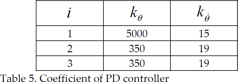
The input variables in the block diagram of the controller (i.e. x_d, ẋ_d, ẍ_d) are outputs of the neural network (i.e. $θ_{1}, {\dot{θ}}_{1}, {\ddot{θ}}_{1}$ ) with the solution of the system of equations with 6 equations (equations of the position, velocity, and acceleration of the end-effector in directions X₀, Y₀) and 6 unknowns that gives $θ_{i}, {\dot{θ}}_{i}, {\ddot{θ}}_{i}, i = 2, 3$ . It is obvious that each torque is a function of $θ_{i d}, {\dot{θ}}_{i d}, {\ddot{θ}}_{i d}, i = 2, 3$ . In addition, the X_d is the set point.

By our experiences and trial and error, the values of coefficients of PD controller are found just as exposed in Table 5.

Table 5.

Coefficient of PD controller

i	$k_{θ}$	$k_{\dot{θ}}$
1	5000	15
2	350	19
3	350	19

For specified values of parameters of mobile manipulator the performance index has been shown in Fig. 7. Tires upward force for tires number 1, 2 has been illustrated in Fig. 8. According to Fig. 8, at the worst case, the difference between two forces is about 2 N which denotes on the correctness of our proposed algorithm.

Fig. 7.

Performance index for a specific case of mobile manipulator when v = 1(m / s), b = 0.5(m), α = 0.5(rad)

Fig. 8.

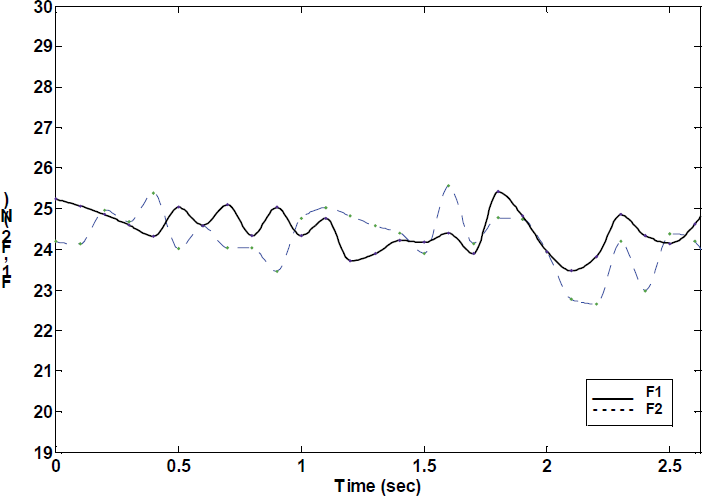
Tires upward force of tires number 1, 2 when v = 1(m / s), b = 0.5(m), α = 0.5(rad)

These values have straight effects on the performance index. A large torque will be created at the beginning of control action. This torque causes the manipulator accelerates. Therefore, this rapid acceleration may cause an increase or decrease in the value of one of tire upward force. If this matter will not be attended, it can be a reason for instability and being tipover. Because of the nature of our system, overturning will be around the transverse axis. Therefore, the PD controller must oppose to this case and turn rapidly the manipulator to the optimum configuration. This effect will be damp within 0.2 first second. Subsequently, the system will be in a better condition such that the tire upward force of two each tire is close together and the controller can swiftly and readily accomplish its duty.

As it is observed in the Fig. 7, in the compensated mobile manipulator, the performance index has a value less than 1 N-m which is well below than the uncompensated mobile manipulator when considered informally for some states of system through motion. It can be expected from this system when the dynamic interaction between the vehicle and manipulator would not exist, the two tire upward forces could be exactly equal to each other. Even though despite existence of those dynamical effects, it can rely on that the mobile manipulator is able to move safely without overturning.

Angular position of manipulator for each joint and for two different conditions when x=0 (at the beginning of motion) and when x=1 (m) (when mobile manipulator moves 1 (m) along × direction) have been demonstrated in figures 9, 10, 11 respect to time history. It should be noted that PD controller will turn the manipulator within 0.2 second. The value for $\dot{θ}$ in equation (11) comes from ${\dot{θ}}_{d e s i r e d}$ of the previous step such that this value guarantees that the end-effector moves with a constant velocity along its path. The value of angular velocities is calculated from the neural network for the case the performance index becomes minimized.

Fig. 9.

Time history of θ¹ for two different positions

Fig. 10.

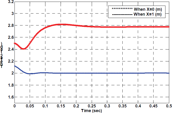
Time history of θ² for two different positions

Fig. 11.

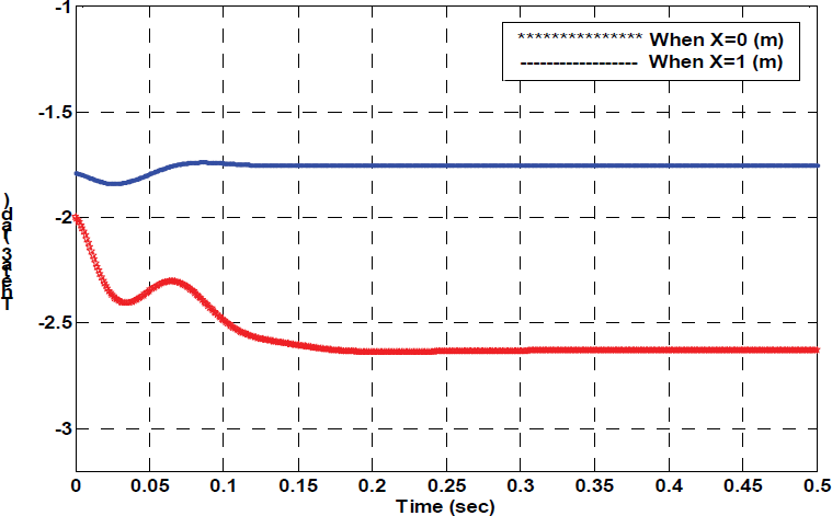
Time history of θ₃ for two different positions

The tracked trajectory by the end-effector is compared to the desired trajectory in Fig. 12. It can be concluded from this illustration that the control algorithm is able to lead the end-effector to the desired trajectory significantly.

Fig. 12.

Comparing the desired and tracked trajectory by the end-effector

5. Conclusion

In this paper, a method is developed for the stability enhancement of mobile manipulators when their vehicle is not large enough to oppose the dynamic effects which come from the motion of manipulator. The proposed method is based on the minimization of a performance index related to the magnitude of the upward forces of vehicle tires. When the forces are all equal, then the performance index is minimized. An extra degree of freedom has been assumed for manipulator so that it can take the best configuration among unlimited arrangements to minimize the performance index. This assumption causes augmentation of complexity of the governing dynamic equations, but the suggested algorithm is able to increase the order of stability of the mobile manipulator significantly. The controlling force is the torque applied on the joint connecting the manipulator to the vehicle. A combination of neural network and genetic algorithm is implemented to derive the appropriate configuration of the system. A PD controller is employed for the closed loop control system. It is shown that with the given algorithm, the upward tire forces are very close in each other and the appropriate positions are attained in a relatively short period of time.

Footnotes

External Iterative Relations

\begin{aligned} ^{i + 1} ω_{i + 1} =_{i}^{i + 1} R^{i} ω_{i} + {\dot{θ}}_{i + 1}^{i + 1} {\hat{Z}}_{i + 1} \\ ^{i + 1} {\dot{ω}}_{i + 1} =_{i}^{i + 1} R^{i} {\dot{ω}}_{i} +_{i}^{i + 1} R^{i} {\dot{ω}}_{i} \times {\dot{θ}}_{i + 1}^{i + 1} {\hat{Z}}_{i + 1} + {\ddot{θ}}_{i + 1}^{i + 1} {\hat{Z}}_{i + 1} \\ ^{i + 1} {\dot{v}}_{i + 1} =_{i}^{i + 1} R (^{i} {\dot{ω}}_{i} \times^{i} P_{i + 1} +^{i} ω_{i} \times (^{i} ω_{i} \times^{i} P_{i + 1}) +^{i} {\dot{v}}_{i}) \\ ^{i + 1} {\dot{v}}_{C i + 1} =^{i + 1} {\dot{ω}}_{i + 1} \times^{i + 1} P_{C i + 1} +^{i + 1} ω_{i + 1} \times (^{i + 1} ω_{i + 1} \times^{i + 1} P_{C i + 1}) +^{i + 1} {\dot{v}}_{i + 1}) \\ ^{i + 1} F_{i + 1} = m_{i + 1}^{i + 1} {\dot{v}}_{C i + 1} \\ ^{i + 1} N_{i + 1} =^{C i + 1} I_{i + 1}^{i + 1} {\dot{ω}}_{i + 1} +^{i + 1} ω_{i + 1}^{C i + 1} I_{i + 1}^{i + 1} ω_{i + 1} \end{aligned}

Internal Iterative Relations

\begin{aligned} ^{i} f_{i} =_{i + 1}^{i} R^{i + 1} f_{i + 1} +^{i} F_{i} \\ ^{i} n_{i} =^{i} N_{i} +_{i + 1}^{i} R^{i + 1} n_{i + 1} +^{i} P_{C i} \times^{i} F_{i} +^{i} P_{i + 1} \times_{i + 1}^{i} R^{i + 1} f_{i + 1} \\ τ_{i} =^{i} n_{i}^{T}^{i} {\hat{Z}}_{i} \end{aligned}

References

Dubowsky

Tanner

A.B.

, “A Study of the Dynamics and Control of Mobile Manipulators Subjected to Vehicle Disturbances”, Proc. IV Inter. Symposium of Robotics Research, Santa Cruz, CA, August 1987.

Dubowsky

Paul

, and West

, “An Analytical and Experimental Program to Develop Control Algorithms for Mobile manipulators”, Proc. VII Symposium of Theory and Practice of Robots and Manipulators, Udine, Italy, September 1988.

“Application of Robotics and Artificial Intelligence to Reduce Risk and Improve Effectiveness: A Study for the United States Army” National Academy Press, Washington, D.C., 1983.

Huang

Sugano

, “Manipulator Motion Planning for Stabilizing a Mobile Manipulator”, Proceedings 1995 IEEE/RSJ Int. Conference, Vol. 3, pp. 467–472, 1995.

Huang

Sugano

, and Tanie

, “Motion Planning for a Mobile Manipulator Considering Stability and Task Constraints”, Proceedings of the IEEE, Int. Conference on Robotics and Automation, Leuven, Belgium, pp. 2192–2198, May 1998.

Huang

Sugano

, and Kato

, “Stability Control for a Mobile Manipulator Using a Potential Method”, Proceedings of IEEE/RSJ Int. Conference on Intelligent Robotics and Systems, Munich, Germany, Vol. 2, pp. 839–846, 1994.

Mitobe

Capi

, and Nasu

, “A New Control Method for Walking Robots Based on Angular Momentum”, Journal of Mechatronics, Vol. 14, pp. 163–174, 2004.

Shiller

Gwo

Y.R.

, “Dynamic Motion Planning of Autonomous Vehicles”, IEEE Transaction on Robotics and Automation, Vol. 7, No. 2, pp.241–249, April 1991.

Meghdari

Naderi

, and Alam

M.R.

, “Tipover Stability Estimation for Autonomous Mobile Manipulator Using Neural Network”, 2004 Japan–USA Symposium on Flexible Automation, JUSFA 2004, Colorado, July 19–21, 2004.

10.

Meghdari

Naderi

, and Eslami

, “Increasing of Stability of Mobile Manipulator Using Dynamic Compensation”, 13^th Annual (International) Mechanical Engineering Conference-May 2005, Isfahan, Iran.

11.

Fleming

P.J.

, and Purshouse

R.C.

“Genetic Algorithm for Control Systems”, IFAC, Professional Brief, Unbehauen

, Oxford, UK, Eoless Publishers, 2004.

12.

Denavit

Hartenberg

R.S.

, “A Kinematic Notation for Lower-Pair Mechanisms Based On Matrices”, Journal of Applied Mechanics, pp. 215–221, June 1955.

13.

Craig

J.J.

, “Introduction to Robotics: Mechanics and Control”, Second Edition, Addison-Wesley, 1989.

14.

Beale

Jackson

, “An Introduction to Neural Network”, Institute of Physics Publishing, Translated by Alborzi

, Sharif University of Technology Publishing, 1998.

15.

Demuth

Beale

, “Neural Network Toolbox for Use with MATLAB”, MATLAB version 7.

Stability Enhancement of Mobile Manipulators via Soft Computing

Abstract

Keywords

Nomenclature

1. Introduction

2. The Dynamic Model of a Mobile Manipulator

Footnotes

External Iterative Relations

Internal Iterative Relations

References