
Abstract
This paper addresses the issues of the Linear Parameter Varying (LPV) modelling and control of flexible-link robot manipulators. The LPV formalism allows the synthesis of nonlinear control laws and the assessment of their closed-loop stability and performances in a simple and effective manner, based on the use of Linear Matrix Inequalities (LMI). Following the quasi-LPV modelling approach, an LPV model of a flexible manipulator is obtained, starting from the nonlinear dynamic model stemming from Euler-Lagrange equations. Based on this LPV model, which has a rational dependence in terms of the varying parameters, two different methods for the synthesis of LPV controllers are explored. They guarantee the asymptotic stability and some level of closed-loop ℒ2-gain performance on a bounded parametric set. The first method exploits a descriptor representation that simplifies the rational dependence of the LPV model, whereas the second one manages the troublesome rational dependence by using dilated LMI conditions and taking the particular structure of the model into account. The resulting controllers involve the measured state variables only, namely the joint positions and velocities. Simulation results are presented that illustrate the validity of the proposed control methodology. Comparisons with an inversion-based nonlinear control method are performed in the presence of velocity measurement noise, model uncertainties and high-frequency inputs.
1. Introduction
The control of robot manipulators is a challenging research area that has attracted the attention of scientists and engineers for several decades (see, e.g., the reference book [1]). In the most basic approaches, the mechanical structure of such articulated systems is assumed to be completely rigid and the control laws are developed based on this hypothesis. The rigidity of the robot can be reinforced by appropriately choosing the building materials, or by treating a posteriori the existing structure. However, due to safety and power consumption constraints, it is often important to keep a light weight. This requirement prevents any structural strengthening, which leads the flexibility effects to remain significant. Lightweight robots that are used in aerospace [2] and medical [3] applications typically exhibit deformable structures. The distributed deformation is referred to as link-flexibility in the field of robotics.
The control of multiple-link flexible manipulators is a difficult problem for several reasons, such as the significance of the nonlinear effects in the dynamic model, the presence of lightly damped oscillatory modes and the underactuated nature of the system (the deformation variables that describe flexibility are neither actuated nor measured). In this context, the end-effector trajectory tracking problem is definitely the hardest to solve. Several works on the subject consider a linearization of the model around a nominal operating condition, or some a priori knowledge of the reference trajectory (see [4], [5] and references therein). Herein, the proposed methodology allows us to deal with the most significant nonlinear effects: the variations of the inertia matrix with respect to the robot configuration and the Coriolis and centripetal torques. The use of deformation sensors, such as strain gauges, accelerometers and optical sensors, is avoided for the sake of the generality of the proposed approach that tackles an output feedback, i.e., a limited information control problem, in which some of the state variables are not measured.
Our goal, in this paper, is to show some of the potentialities offered by the Linear Parameter Varying (LPV) systems methodology for the control of flexible-link manipulators. Some of the advantages of this methodology are its validity for systems undergoing unstable zero dynamics and its ability to guarantee performance and robustness properties, due to the tuning in the frequency domain. Therefore, LPV methods have become increasingly popular in robotic applications, starting from the results presented in [6], where the Coriolis and centripetal nonlinearities were not considered. More recently, the work in [7] used a conservative affine LPV model which is reduced using parameter set mapping. The work presented in [8] used an identified polynomial LPV model and carried out robust performance analysis using matrix sum of squares relaxations. Herein, an LPV model with rational parametric dependence is considered. This rational dependence is caused by the nonsingular descriptor structure of mechanical systems.
As a first step towards the design parameter-dependent control laws, an appropriate LPV model of the system must be derived. The LPV modelling procedure can be carried out in two ways. 1) A direct identification from experimental data, knowing the structure and the type of the parametric dependence of the LPV model. 2) A reformulation of the nonlinear dynamic model obtained from multibody dynamics. The work presented in this paper follows the second approach. Among the various methods of LPV modelling of physical systems [9], we have adopted the virtual scheduling change-of-variable one. It consists in directly reformulating some nonlinear terms that involve the measured states as varying parameters. This is consistent with our application because the involved models have a relatively small number of different types of nonlinearity.
The type of parametric dependence of the state matrices in terms of the varying parameters plays a key role in the numerical tractability of the controller synthesis problem. For instance, the rational dependence may lead to an infinite dimensional Linear Matrix Inequality (LMI, see [10]) optimization problem that is difficult to handle numerically. Moreover, considering that the state variables that describe the deformations are unmeasured, this prevents the direct use of a state feedback controller. In such a situation, one may consider an observer-based control scheme or a dynamic output feedback (DOF) method. The latter has been adopted in our work because in this case, the performance requirements are easier to manage at the controller synthesis stage.
In order to address the above-mentioned control design issues and to synthesize LPV-DOF controllers that ensure the internal stability and some level of ℒ2 -gain performance over a wide operating range, we propose the following two different approaches:
The use of an equivalent affine LPV descriptor model that represents the original rational LPV one. The use of some dilated LMI conditions that exploit the nonsingular descriptor structure of the LPV model.
Both methods finally allow us to simplify the rational dependence of the LMI synthesis conditions and to obtain affine parameter-dependent LMIs (PDLMIs) that can be solved on the vertices of the parametric space.
The paper is organized as follows. The second section introduces some preliminaries and states the addressed problem. Section 3 deals with the nonlinear and the LPV modelling of flexible manipulators. The proposed control strategies are presented in Section 4. Section 5 is devoted to the implementation of the control laws on a system taken from the literature and presents some simulation results. In the sixth section, comparisons with an optimized inversion-based control law are conducted and Section 7 concludes the paper.
Notations - If A and B are symmetric matrices A > 0 (resp. ≥ 0) means that A is positive definite (resp. positive semi-definite), A < 0 means that A is negative definite, A
T
is the transpose of A, He A = A + A
T
,
2. Preliminaries and problem statement
First of all, let us define the following variables: θ(t):
vector of measured angular positions (rigid coordinates), θ*(t): vector of joint reference trajectories,
δ(t): vector of unmeasured deflection variables (flexible coordinates),
F(t) = [X(t) Y(t)] T : vector of end-effector position variables in the plane (Cartesian coordinates),
F*(t): vector of end-effector reference positions,
Λ−1 (θ): inverse kinematics of the robot, i.e., the relation between the configuration variables θ and the operational variables F.
Robot manipulators are generally used in order to perform a task that is often expressed in the operational space (i.e., the end-effector space). As the actuation takes place at the joint level via the use of motors, the task to be performed needs to be translated into the joint space by using the inverse kinematics of the robot. The computation of the joints' reference trajectories θ* can be performed off-line if the task is known in advance or is repetitive. Otherwise, it must be updated in real-time. In our work, we suppose that the measured variables are the joint angular positions θ(t) and velocities
According to the previous hypotheses, Figs. 1 and 2 represent the joint space and the operational space control schemes in the case of flexible manipulators. The quasi-LPV controller K̂(ρ), where

Joint space control scheme

Operational space control scheme
The methodology presented in this paper focuses on the control scheme of Figure 1 while managing the most significant nonlinear effects such as the Coriolis and centripetal effects. Let us note, however, that this methodology can also be applied for direct operational space control, but an increase of the number of state variables and varying parameters is then expected.
3. Modelling of flexible manipulators
Robot manipulators can undergo two main classes of flexibilities [5]: joint flexibility that is concentrated at the joints of the manipulator and may be caused by the use of compliant transmission elements, and link flexibility that is distributed along the mechanical structure and may be caused by the use of lightweight materials or the excitation by high-bandwidth input torques. Our paper focuses on the link flexibility case which is the most challenging one. A robotic manipulator with two joints and a flexible forearm (second link) is considered as a case study.
3.1. Dynamic modelling
3.1.1. Modelling of the bending deflection
The assumed modes technique is a common approach for the modelling of the deformation occurring in a flexible link. Under the hypothesis of small deformations of pure bending nature, the deformation varies with respect to the position x k ∈ [0, l k ] in the k th link according to the formula:
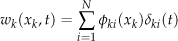
where l k is the length of the link, Φ ki (x k ) the shape of its i th flexible mode, (t) its time-varying amplitude and N is the number of considered flexible modes per link. The most common expressions of mode shapes are polynomial [12] and trigonometric functions [13]. Their coefficients are determined by imposing some boundary conditions on the deformation. For instance, in the clamped-free boundary conditions, the first extremity of the link is fixed to the base with a zero tangent slope whereas this slope is nonzero in the pinned-free ones. The second extremity of the link is not constrained in both cases.
3.1.2. Nonlinear dynamic model
The equations of motion are obtained following the usual Euler-Lagrange approach, leading to the dynamic model:

This model exhibits a second-order behaviour in terms of the vector of generalized coordinates q = [θ
T
δ
T
]
T
. The inertia, stiffness and damping matrices are partitioned following the rigid-body and flexible variables as:
3.2. Case study
The case study discussed in our paper is the model of the FLEXARM robot taken from [15]. A schematic view of this flexible manipulator is displayed in Figure 3.
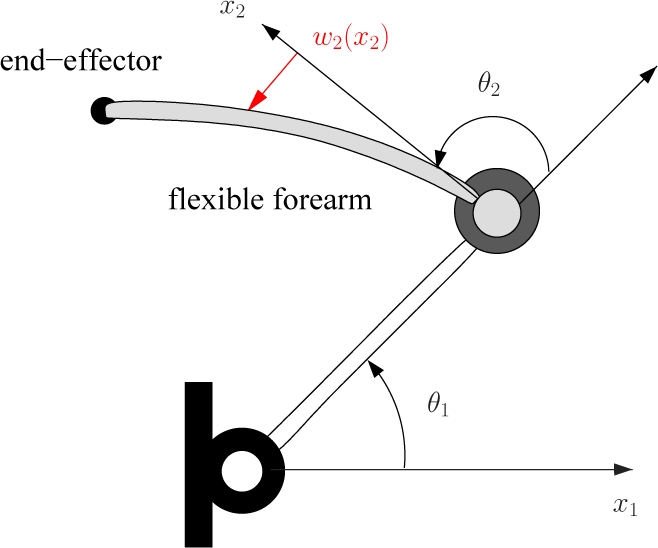
Schematic view of the flexible manipulator
3.2.1. Nonlinear model
The considered robot is a planar 2-link manipulator with a flexible forearm. The lengths of its links are: l1 = 0.3 m and l2 = 0.7m. Its nonlinear dynamic model is given by (2), where q(t) = [θ1(t) θ2(t) δ21(t) δ22(t)] T , θ1,2(t) being the joint angular positions and δ2j(t), j = 1,2, the amplitudes of the two considered flexible modes with trigonometric shaping functions and clamped-free boundary conditions. The inertia matrix has the following expression:

where:

J1t, J2t, h1 h2 and h3 are the contributions of the different elements (rigid bodies, rigid-flexible couplings) to the moments of inertia.
The Coriolis and centripetal torques are quadratic terms of the time-derivatives of the generalized coordinates. Their expressions can be developed from the inertia matrix M(q) using the Christoffel symbols [16]. The components of the vector C(q, q̇)q̇ are:

The input matrix is:
where
3.2.2. LPV model
In order to obtain a relevant LPV model for system (2), the terms involving the deformation variables δ2j, j = 1, 2, are neglected in the inertia matrix. Indeed, their effect is insignificant when they are added to the rigid parts of the moments of inertia. It is not the case in the Coriolis vector where they must be considered. Then, it appears that M(q) and c(q, q̇) can be written as a linear combination of the following varying parameters, that involve the measured state variables of the system:

Each parameter ranges between known extremal values, as well as its time-derivative:


The boundaries of these admissible sets are respectively delimited by the following vertices sets:


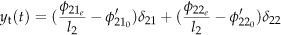
Taking the regulated output of the system as the joint angular positions yields the following descriptor model:

where: M1(ρ) = diag(I4, M(ρ)), C = [I2 02×6],

The parameter-dependent entries of the matrix S(p) are simply obtained by factoring the components of the Coriolis vector. For instance, S[33](ρ) = h1ρ3 is obtained by recognizing that
By passing M1(ρ) through the right-hand side, the model in (10) can be written in the usual state-space form:

where
Due to the inversion of the inertia matrix M(p) in the state matrices A(ρ) and B(ρ), the LPV system (11) is rational with a particular structure. Indeed, the state matrices are already factored in a Denominator−1 × Numerator form in a matrix sense.
4. LPV control strategies
4.1. Controller synthesis problem
Let us provide the LPV model G(s,p) with a performance channel whose input is
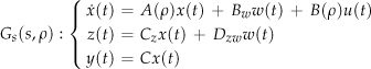
The LPV-DOF control problem is to synthesize a controller of the form:
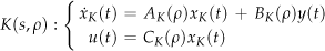
such that the closed-loop system defined by:

where xCl=[xT xKT] T , is asymptotically stable and satisfies a level of ℒ2. -gain performance over the parametric set &Scr; ρ .
The ℒ2-gain of the closed-loop system is defined as:

4.2. Equivalent affine LPV descriptor representation
It has been stated in [18] that any rational LPV system can be expressed in a descriptor form with affine state matrices. Let us summarize, hereafter, some technical aspects of the method.
4.2.1. Modelling
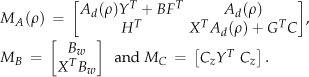
In the general case, a rational LPV system is described by the state-space equation given in (11), in which the state matrices A(ρ), B(ρ) and potentially the output matrix C(ρ) are rational functions of the parameter vector ρ(t). Transforming model (11) into an affine descriptor model can be performed either by making some changes of variables involving the parameter-dependent entries of the state matrices (ad-hoc methods), or systematically by using a Linear Fractional Representation (LFR) modelling of the system. The LFR model itself can be obtained by manual calculations or by using available numerical software [19]. It is characterized by the feedback interconnection of a Linear Time-Invariant (LTI) system and a parameter-dependent matrix Δ(ρ):

and v(t) = Δ(ρ)z d (t)
where x(t) ∈ ℝ
r
is the state,
C
d
= [N31 0] and D
zw
= N22. Note that the alternative choice: x
d
(t) = [x
T
(t) v
T
(t) u
T
(t)]
T
for the generalized state vector yields a constant B
d
matrix.

4.2.2. ℒ2-gain control
The following theorem gives some controller synthesis conditions for the affine LPV descriptor model (17).
Theorem 1. [18] The closed-loop system is stable and the ℒ2-gain from w(t) to z(t) is less than γ > 0 if the LMIs (18)–(19) have a solution p = {X, Y, F, G, H},


where:
The LPV controller is directly obtained in the regular state-space form (13) (see [18]). The synthesis conditions of Theorem 1 are obtained based on a generalized version of the bounded real lemma theorem [10] to descriptor systems [21].
4.3. Dilated LMI conditions and structure constraints
The dilated LMI conditions involve, besides the usual Lyapunov, controller and plant matrices, some additional matrix variables referred to as slack variables. These variables offer additional degrees of freedom for the analysis and the synthesis problems. For instance, Parameter-Dependent Lyapunov Functions (PDLF) can be considered, which results in a reduction of the conservatism caused by the use of a single Lyapunov function, as explained in [22].
The following ℒ2-gain analysis conditions, given in [23], are based on the dilated LMI conditions proposed in [24].
Theorem 2. The closed-loop system (14) is stable and the ℒ2-gain from w(t) to z(t) is less than γ > 0 if ∃P(ρ) = P
T
(ρ) (Lyapunov matrix) and ∃V (slack variable) solutions of the LMI (20),

We are now ready to introduce our main synthesis result that is stated in the following theorem.
Theorem 3. There exists a controller (13) that stabilizes the closed-loop system (14) and achieves an ℒ2-gain less than γ > 0 if the LMI (21) has a solution
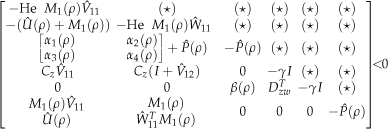
where:
The state matrices of the controller are then given by:
Proof: Starting from the following partitioning of the slack variable and its inverse, according to the dimensions of the system and the controller:
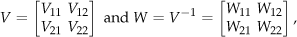
some linearizing projections are defined as:

Let us now introduce the following transformation matrix T(ρ), where M 2 (ρ) = diag(M1(ρ), I8):

Keep in mind also that the closed-loop state matrices in (14) are partitioned as:
The synthesis conditions of Theorem 3 are obtained by left multiplying the analysis inequality (20) by T(ρ) and right multiplying by its transpose (congruence transformation), then making the changes of variables:
Remark 1. From the solution of the LMI (21), the matrices W21 and V21 used in the controller formula are obtained by performing a factorization of the right-hand side of
Remark 2. The analysis conditions of Theorem 2 are independent from the type of the parametric dependence of the system G
Cl
(s, ρ) in (14). If the state matrix A
Cl
(ρ) is affine, it is equivalent to solve the PDLMI (20) on the set of vertices
Remark 3. In order to facilitate the numerical tractability of the controller synthesis conditions of Theorem 3, the parameter-dependent matrices Û(ρ) and
5. Implementation
5.1. Control issue
The descriptor and the dilated LMI controller synthesis methods have been implemented in simulation for the control of the FLEXARM robot. In particular, the control scheme presented in Figure 4, that contains a 2-block performance channel, has been adopted. The vector of external inputs consists of the joint references w(t) = θ* (t). The vector of controlled outputs,

H∞ control scheme
5.2. Simulation results
Time simulations have been carried out in order to evaluate the proposed control methods. Let us define the following limits that generate the admissible set S ρ : ρ1 ≤ 1 (by definition of the cosine function), ρ2, ρ3 ≤ 0.3 rad/s, and ρ4, ρ5, ρ6 ≤ 0.045 (rad/s)2. These bounds are set so as to guarantee some relatively high performance levels. While the stability of the closed-loop system is ensured over the whole admissible set, the performance indices presented in the paper are guaranteed for ρ1 ≤ 0.5. Let us point out that the LPV controllers can operate outside the admissible parametric set, but a degradation of the performance is then expected. In order to provide a tighter estimate of the actual operating range, a usual approach is to perform an a posteriori performance analysis, by fixing the controller matrices and computing the performance level for different parametric sets.
The control problem of Figure 4 has been addressed using both proposed LPV methods. The LMI conditions (18)–(19) and (21) have been solved on the vertices set
In the sequel, we present some simulation results using the weighting functions W1(s) = 1 and W2 (s) = 0.1. Static functions are employed herein so as to avoid an increase of the order of the system. The obtained performance indices are γ = 2.37 and γ = 2.10 for the descriptor and the dilated LMI synthesis conditions, which guarantees a modulus margin of
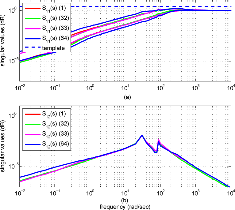
Realized frequency transfers (descriptor method)
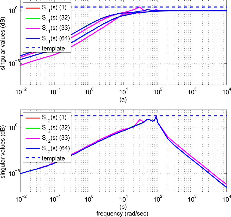
Realized frequency transfers (dilated LMI method)
The joint reference signals θ*1(t) and θ*2(t) are designed so as to assess the accuracy of the tracking and the decoupling of the two joints over the whole operating range. Smooth signals are involved in order to meet the limitations on the parameters. Figs. 7-(a) and 8-(a) show the time-responses of the closed-loop system obtained with the original nonlinear model and the LPV controller. Figs. 7-(b) and 8-(b) display the corresponding trajectory tracking errors. Figs. 9 and 10 present the time evolution of the varying parameters for both methods. The presented Figures demonstrate the effectiveness of the LPV methods in preserving the closed-loop system stability and performances over a wide operating range.

Tracking of the reference trajectories (descriptor method)
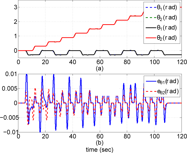
Tracking of the reference trajectories (dilated LMI method)

Evolution of the parameters (descriptor method)

Evolution of the parameters (dilated LMI method)
In addition to the previous control theory-oriented test, a practice-oriented simulation test has been made in order to assess the trajectory tracking in the Cartesian space. The end-effector of the robot has to follow a rectangular trajectory F*(t) = (X*(t), Y*(t)), starting from the position (X, Y) = (0.2121 m, 0.9121 m) that corresponds to the unstable equilibrium position (θ1,θ2) = (45°,45°). Figs. 11-(a) and 11-(b) show the time tracking of the X and Y coordinates respectively. Figure 11-(c) shows the tracking in the Cartesian plane (X, Y) . The subscripts 1 and 2 in the legends indicate the descriptor and the dilated LMI method respectively.
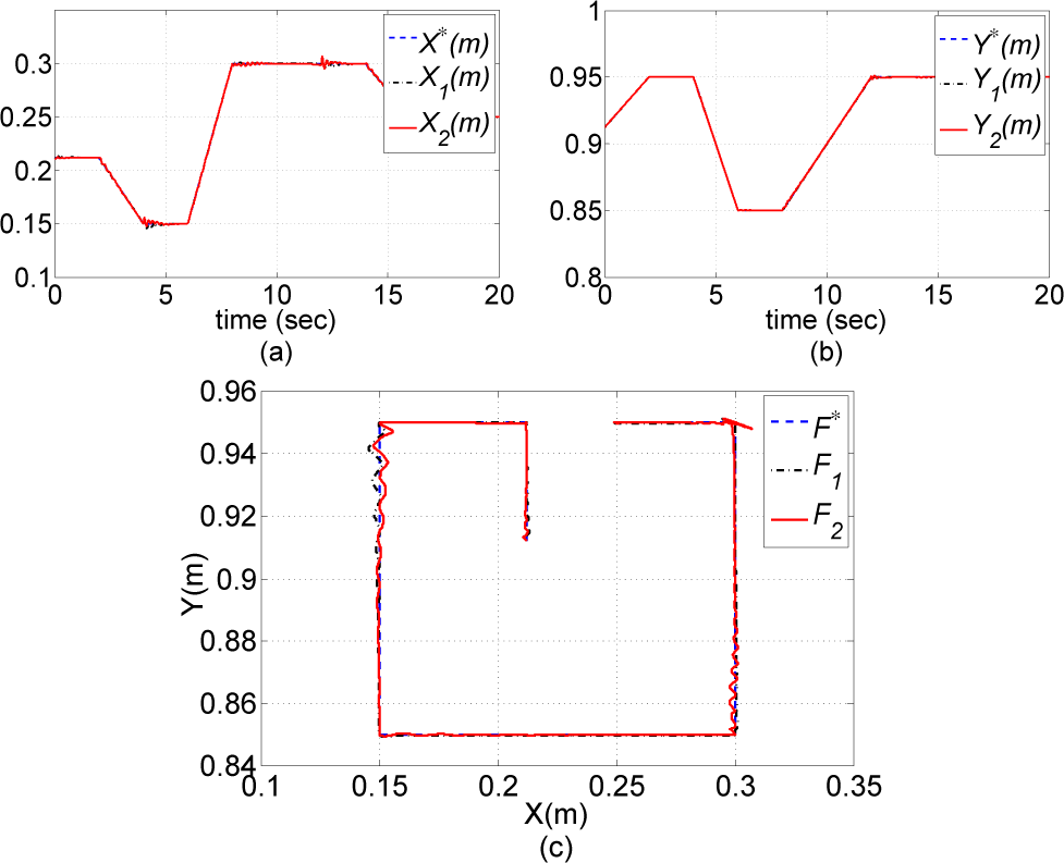
Trajectory tracking in the Cartesian space - (a): X coordinate, (b): Y coordinate, (c): (X, Y)-plane
Remark 4. When a min-max description of the parametric space is used, as in (6)–(7), the number of LMI constraints that need to be solved increases exponentially with the number of varying parameters. This fact may constitute a limitation for systems with a large number of parameters. Nevertheless, this issue can be addressed by following an alternative representation of the parametric space, such as the use of semialgebraic sets together with a generalized version of the S-procedure theorem [8]. This approach leads to a single parameter-independent LMI of larger size.
6. Comparison with a nonlinear inversion-based control approach
The nonlinear inversion-based control method is very popular in robotics. In the following, we present a comparison of this method with the proposed LPV dilated LMI method.
6.1. Basic knowledge on inverse dynamics control
The principle of the method is to apply a nonlinear state feedback τ = ψ(q, q̇) in equation (2) in order to obtain a linear and decoupled tracking error dynamics (see, e.g., [16]). The control input may be taken as:

A simple choice for the auxiliary control input v is:

where q* is the vector of reference trajectories of the generalized coordinates. Following (23)–(24), the dynamics of the tracking error eq = q* − q is:
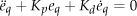
The diagonal structure of matrices Kp and K d results in a decoupling of the error dynamics and their positive definiteness ensures the asymptotic cancellation of e q . Robustness with respect to model uncertainties has been addressed in [16, 27].
6.2. Extension to flexible manipulators
The inversion-based control scheme described in (23)–(24) is built on the assumption that the state vector x = [q
T
q̇
T
]T is entirely measurable. However, in the case of flexible manipulators, such a control structure is not exploitable because the deformation variables δ and
The feedforward part τ N of the control is the torque needed to exactly reproduce the joint reference trajectory θ*(t) based on a perfect knowledge of the model of the robot. The feedback part τ PD , e.g., of proportional and derivative (PD) nature as in (24), is used to provide some robustness against model uncertainties. The overall control law is then:

Let us describe more precisely this control law. The presented developments are borrowed from [13]. Setting g(q) = 0 and M δδ = I in (2), the deformation variable equation becomes:
where
Replacing this expression of

where H = I − M θδ G δ .
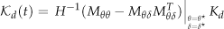
Let us now follow a model inversion approach and replace

Therefore, the control torque in (28) takes the composite form in (26), where:


with:

The feedforward part τ
N
of the control law depends only on the reference trajectories and the model of the system. The rigid-body reference signals θ*,
6.3. Comparative study
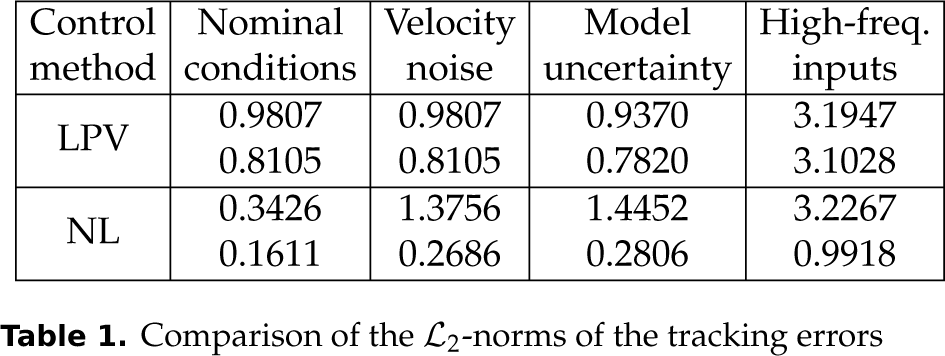
It is difficult to make a fair comparison between two methods that are so different in nature. In the comparison presented in the following, strong efforts have been made in order to obtain the best results with the inversion-based method. Constant feedback gains K p and K d can be designed so as to achieve some performance properties. For instance, the pole placement technique is used to set the damping ratio and the natural frequency of the tracking error dynamics. For our application, this tuning yielded degraded performances compared to the LPV method. Better results were obtained using recently developed tools that are based on nonsmooth optimization [28]. They allow synthesizing structured and fixed-order controllers for linear systems. The main tool is the hinfstruct function of MATLAB [29], devoted to H∞ synthesis. We have performed a synthesis using a linearized model of the system around the nominal value x = 0 of the state vector. We minimized the H∞ norm of the sensitivity function weighted by a filter that imposes the following performance features: a modulus margin of 0.8, a bandwidth of 1 rad/s and a static position error of 5%. The obtained performance index is γNS = 1.48 and the feedback gains are: K p = diag(18.75,19.55) and K d = diag(3.70,4.60).
Both the LPV and the inversion-based controllers exhibit a satisfactory behaviour in nominal operating conditions (as described in Section 5.2). However, the LPV controller has proven to be more robust in challenging ones. Among the various comparative tests conducted, the results obtained in the three following situations allowed some discrimination.
A uniformly distributed pseudo-random noise on the joint velocity measurement whose amplitude is ±25% of the nominal value. A time-varying uncertainty on the moments of inertia of 15% of their nominal value. This uncertainty can for instance represent an unknown time-varying load. It is implemented in simulation as a pseudo-random noise. Faster steps for the reference inputs θ*: settling time of 0.5 s instead of 3 s.
The columns of Figs. 12–13 gather the results obtained in these three operating conditions respectively. Their rows represent the time and frequency-domain (Fast Fourier Transform) descriptions of the control input u(t) = τ(t). While the tracking of the reference trajectories is accurate with both control methods, the Figures show that the control input delivered by the LPV controller is much smoother in all cases, whereas a significant oscillating behaviour is observed with the inversion-based controller. Figure 13-e shows that the application of a high-frequency input with this controller excites the resonances of the flexible modes, unlike the LPV controller (Figure 12-e) that significantly attenuates them.
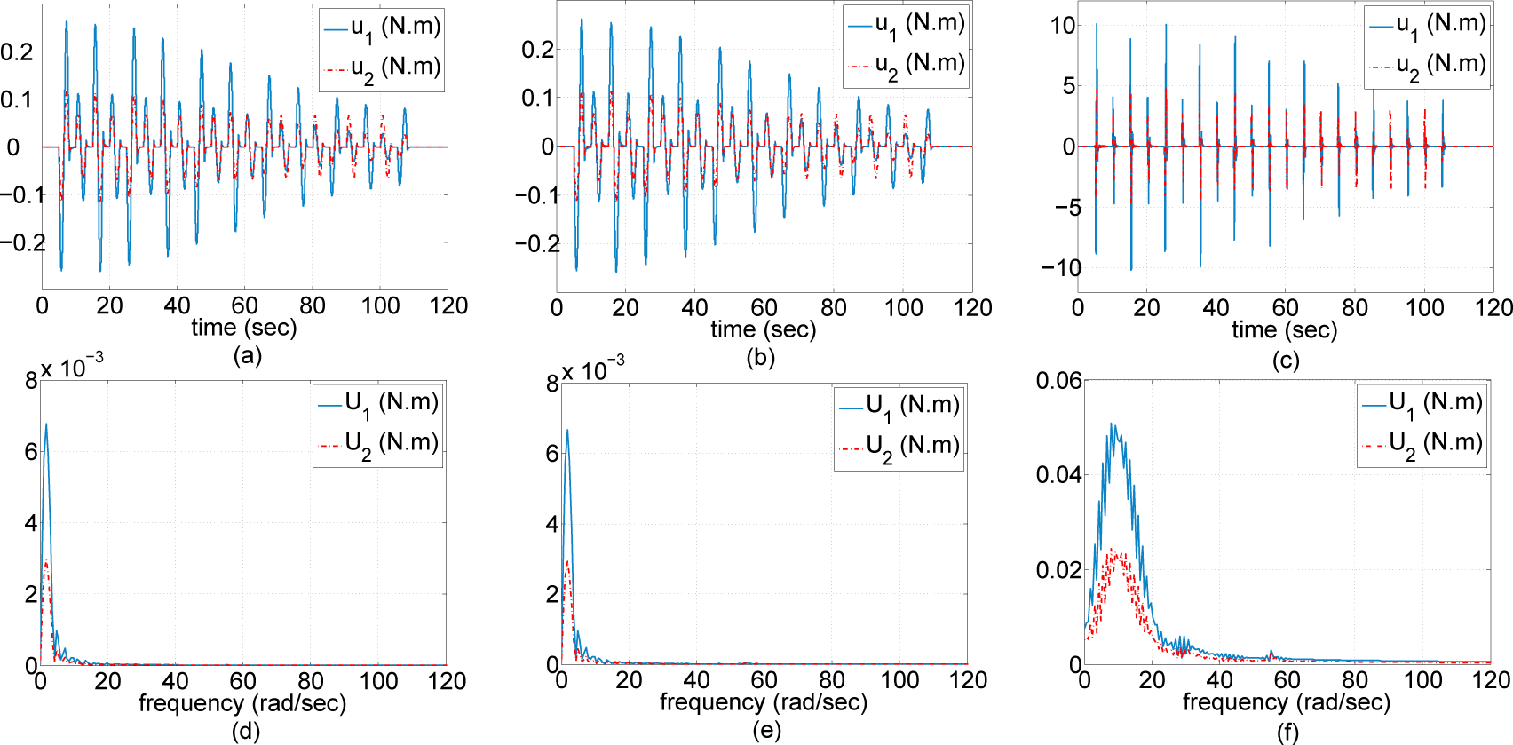
Robustness evaluation of the LPV control method: (a) & (d): velocity noise, (b) & (e): model uncertainty, (c) & (f): high-frequency inputs
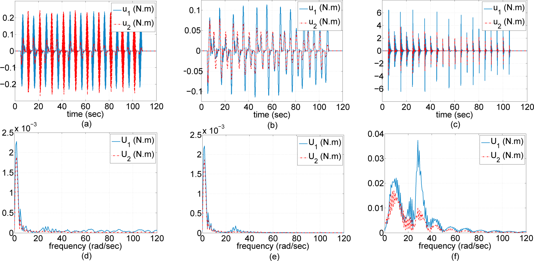
Robustness evaluation of the inversion-based control method
Further analysis results have been obtained for the three tests. In Table 1, the ℒ2-norms of the joint tracking errors
Comparison of the ℒ2-norms of the tracking errors
7. Conclusion
In this paper, we propose a methodology for the modelling and the control of flexible robot manipulators using the Linear Parameter Varying (LPV) systems framework. The smooth nonlinear effects of the dynamic model are handled following a quasi-LPV modelling approach. Two synthesis methods that deal with the rational parametric dependence of the system are investigated, namely the descriptor systems method and the dilated LMI method. Comparisons with a nonlinear inversion-based control technique are provided in the presence of measurement noise, high-frequency inputs and model uncertainty. They illustrate the effectiveness and the robustness of the proposed LPV control methodology.