Sage Journals: Discover world-class research

Abstract

A real world environment is often partially observable by the agents either because of noisy sensors or incomplete perception. Moreover, it has continuous state space in nature, and agents must decide on an action for each point in internal continuous belief space. Consequently, it is convenient to model this type of decision-making problems as Partially Observable Markov Decision Processes (POMDPs) with continuous observation and state space. Most of the POMDP methods whether approximate or exact assume that the underlying world dynamics or POMDP parameters such as transition and observation probabilities are known. However, for many real world environments it is very difficult if not impossible to obtain such information. We assume that only the internal dynamics of the agent, such as the actuator noise, interpretation of the sensor suite, are known. Using these internal dynamics, our algorithm, namely Kalman Based Finite State Controller (KBFSC), constructs an internal world model over the continuous belief space, represented by a finite state automaton. Constructed automaton nodes are points of the continuous belief space sharing a common best action and a common uncertainty level. KBFSC deals with continuous Gaussian-based POMDPs. It makes use of Kalman Filter for belief state estimation, which also is an efficient method to prune unvisited segments of the belief space and can foresee the reachable belief points approximately calculating the horizon N policy. KBFSC does not use an “explore and update” approach in the value calculation as TD-learning. Therefore KBFSC does not have an extensive exploration-exploitation phase. Using the MDP case reward and the internal dynamics of the agent, KBFSC can automatically construct the finite state automaton (FSA) representing the approximate optimal policy without the need for discretization of the state and observation space. Moreover, the policy always converges for POMDP problems.

Keywords

POMDP Stochastic Control Finite State Automata Markov Decision Process

1. Introduction

Traditional learning approaches deal with models that define an agent and its interactions with the environment via its perceptions, actions, and associated rewards. The agent tries to maximize its long term reward when performing an action. This would be easier if the world model was fully observable, namely the underlying process was a Markov Decision Process (MDP). However, in many real world environments, it will not be possible for the agent to have complete perception. When designing agents that can act under uncertainty, it is convenient to model the environment as a Partially Observable Markov Decision Process (POMDP). This model incorporates uncertainty in the agent's perceptions that have continuous distributions, actions and feedback which is an immediate or delayed reinforcement. POMDP models contain two sources of uncertainty; stochasticity of the controlled process, and imperfect and noisy observations of the state (Kaelbling et al. 1996).

In POMDPs, a learner interacts with a stochastic environment whose state is only partially observable. Actions change the state of the environment and lead to numerical penalties/rewards, which may be observed with an unknown temporal delay. The learner's goal is to devise a policy for action selection under uncertainty that maximizes the reward. Although, the POMDP framework is useful in practically modeling a large range of problems, it has the disadvantage of being hard to solve, where previous studies have shown that computing the exact optimal policy is intractable for problems with more than a few tens of states, observations and actions. The complexity of POMDP algorithms grows exponentially with the number of state variables, making it infeasible for large problems (Boyen and Koller 1998, Sallans 2000). Most of the methods dealing with POMDPs assume that the underlying POMDP parameters are known. However, collecting such information is impossible for most of the real world cases. Additionally, past work has predominately studied POMDPs in discrete worlds. Discrete worlds have the advantage that distributions over states (so called “belief states”) can be represented exactly, using one parameter per state. The optimal value function (for finite planning horizons) has been shown to be convex and piecewise linear, which makes it possible to derive exact solutions for discrete POMDPs (Kaelbling et al. 1996).

In this study we aim to use POMDP as a model of the real environment. Since discrete case POMDPs are hard to solve, many studies focus on these type of problems. But the application of such algorithms to robotics which are continuous in nature is nearly impossible. There are a few studies on continuous POMDPs. Recently two studies have been presented. Vlassis, Porta and Spaan, in their work, assume discrete observation over continuous state space (Porta et al. 2005). Hoey and Poupart assume discrete state space with continuous observation (Hoey and Poupart 2005). In these two studies, they further assume that the world model is given. We have made two assumptions that do not exist in nearly none of the previous studies. First, we assumed that the POMDP parameters or world dynamics, such as observation and transition probabilities, are not known, and we expect our agent, simply using its internal dynamics, to generate an optimal policy by making an approximation to exact value function over belief space. Second, since a large number of real world problems are continuous in nature, we are interested in POMDP's with continuous parameters which cannot be solved exactly.

In section 2 we formally describe conventional POMDP solution techniques. In section 3 we describe Kalman Based Finite State Controller (KBFSC)-Learning algorithm in detail. In section 4 we give the experimental results for some well-known POMDP problems. We conclude in section 5.

2. POMDP and Conventional Solution Techniques

POMDPs contain two sources of uncertainty: the stochasticity of the underlying controlled process, and imperfect observability of its states via a set of noisy observations (Sondik 1978). Noisy observations and the ability to model and reason with information gathering actions are the main features that distinguish the POMDPs from the widely known Markov decision process (MDP).

The formal definition of a POMDP is a 6 tuple (S, A, θ, T, O, R) where;

S is the set of states,

A is the set of actions,

θ is the set of observations,

R is the reward function S × A → R,

O is the set of observation probabilities that describe the relationships among observation states and actions S × A × θ → [0,1],

T is the state transition function S × A → Π(S), where a member of Π(S) is a belief state that is a probability distribution over the set S.

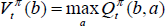
The immediate rewards, received when the agent takes an action at any given belief state, are fed in order to give hint to the agent about what is right and what is wrong. The goal of a POMDP agent is to optimize the expected discounted reward that is the discounted infinite sum of instant rewards, given in Eq. 1.

E (\sum_{t = 0}^{\infty} γ^{t} r (t))

(1)

The methods for learning within the POMDP (Kaelbling et al. 1996) framework may be classified as exact but intractable methods and approximate methods. There are two versions of the POMDP training problem: learning when a model of the POMDP is known, and the much harder problem, learning when a model is not available. Obtaining the world dynamics for complex environments is very difficult. Since the final policy is built on world dynamics, a wrong or idealized world model will lead to poor policies which will cause serious problems in real world environments. Therefore, most of the suggested solution techniques for discrete state space POMDPs where the world model is given are not appropriate for robotics in which world dynamics can not be calculated exactly and is continuous in nature.

Recently two studies, one assuming discrete observation over continuous state space (Porta et al. 2005) and one assuming discrete state space with continuous observation space (Hoey and Poupart 2005) have been presented. Although, they assume that the world model is given, both of them use point based value iteration technique (Pineau et al. 2003) for Gaussian-based POMDPs. Point based value iteration (PBVI) is an approximate solution technique that requires belief point backups chosen based on a heuristic. The solution is dependent on the initial belief and, need a time consuming belief point set expansion and pruning phase for α-vectors.

2.1. Kalman Filters

In the POMDP approaches, the agent's state is not fully observable; the agent tries to convey uncertain or incomplete information about the state of the world. The agent remembers past observations up to some finite number of observations, called a history denoted by the set, {h_t−1, h_t-2, …, h_t-n}.

Astrom (Astrom 1965) conceived an alternative to storing histories: belief state, which is the probability distribution over the state space, S, summarizing the agent's knowledge about the current state. The belief state is sufficient in the sense that the agent can learn the same policies as if it had access to history (Kaelbling et al. 1996).

\sum_{s \in S} b_{t} (s) = 1

Here b_t(s) is the probability that the world is in state s at time t. Knowing b_t(s) in Eq. 2, an action, a and an observation, o, the successor belief state can be computed by Eq. 3.

b_{t + 1} (s) = \frac{\sum_{s} b_{t} (s) P (s^{'} ∣ s, a) P (o ∣ s, a, s^{'})}{\sum_{s, s^{'}} b_{t} (s) P (s^{'} | s, a) P (o ∣ s, a, s^{'})}

(3)

Eq. 3 is equivalent to Bayes filter, and its continuous case forms the basis of Kalman filters (Howard 1960).

The Kalman filter (Grewal and Andrews 1993, Maybeck 1979) addresses the general problem of trying to estimate the state of the agent. Nearly all algorithms for spatial reasoning make use of this approach.

The Kalman filter is a recursive estimator. This means that only the estimated state from the previous time step, action and the current measurement are needed to compute the estimate for the current state. In contrast to batch estimation techniques, no history of observations and/or estimates is required. A belief state is represented by Kalman filter with a mean, the most probable state estimation and a covariance, the state estimation error.

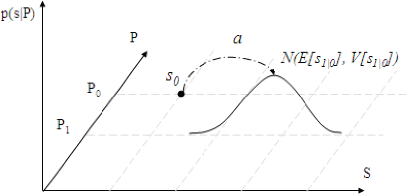
The graphical representation of POMDPs is given in Fig. 1. The Kalman filter relates the current state, s_t, to previous state, s_t−1, and action a_t−1, disturbed by actuator noise using a state transition equation. Tikewise, the observation o_t is a function of the current state and disturbed by sensor noise. Both the actuator and the sensor suite of real world agents are subject to some noise. Kalman assumes that these are Gaussian as given in equations 4 and 5. In practice, the process noise (v) covariance, Q, and measurement noise (n) covariance, R, matrices might change with each time step or measurement, however in this research we assume that they are constant.

p (v) \sim N (0, Q)

(4)

p (n) \sim N (0, R)

(5)

Fig. 1.

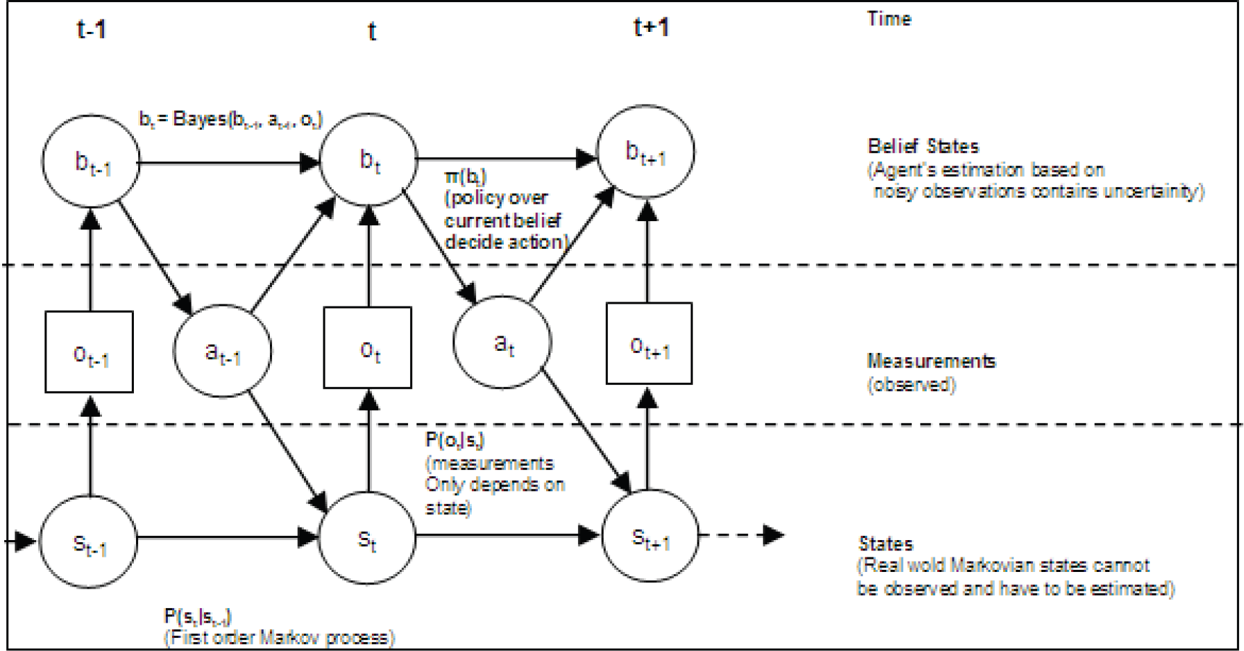
Graphical representation of POMDPs.

In this research, we have linearized the motion model. The general linearized motion model equation is given in Eq. 6.

s_{t} = A s_{t - 1} + B a_{t - 1} + v_{t - 1}

(6)

Likewise, we have also linearized the sensor model. The general linearized sensor model equation is given in Eq. 7.

o_{t} = H s_{t} + n_{t}

(7)

The matrix A in Eq. 6 relates the state at the previous time step to the state at the current step, in the absence of either a driving function or process noise. Note that in practice A might change with each time step, but here we assume it is constant. The matrix B relates the optional control input to the state s. The matrix H in Eq. 7 relates the state to the measurement o. In practice H might change with each time step or measurement, but in this research we assume that it is also constant.

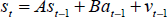
To compute the minimum mean square error estimate of the state and covariance, the following equations are used. The estimate of the state variables,

s_{t | t - 1}^{^{-}} = A s_{t - 1} + B a_{t - 1}

(8)

Where the subscript (t\t − 1) denotes that the value at time step t is predicted using the value at time t−1. The estimate of the sensor reading,

o_{t | t - 1} = H s_{t | t - 1}

(9)

The covariance matrix for the state P,

P_{t | t - 1} = A P_{t - 1} A^{T} + Q

(10)

Kalman filter calculates parameters of a Gaussian distribution, the mean representing the most probable state and the covariance representing the uncertainty. In our study, recursively calculated Gaussian distribution represents a belief state. At each time step, the state and covariance is calculated recursively. This feature matches the belief state defined by Astrom (Astrom 1965), as a sufficient statistic representing the whole history. The Kalman filter divides these calculations into two groups: time update equations and measurement update equations. The time update equations are responsible for projecting forward (in time) the current state and error covariance estimates to obtain the priori estimates for the next time step. The measurement update equations are responsible for the feedback, i.e. for incorporating a new measurement into the priori estimate to obtain an improved posteriori estimate. The final estimation algorithm resembles that of a predictor-corrector algorithm as shown below in Fig. 2.

Fig. 2.

The recursive structure of Kalman Filter

The specific equations of time update functions are given in Eqs. 8 – 10, and the specific equations of measurement update functions are as follows:

K_{t} = P_{t}^{^{-}} H^{T} (H P_{t}^{^{-}} H^{T} + R)^{- 1}

(11)

s_{t} = s_{t}^{^{-}} + K_{t} (o_{t} - H s_{t}^{^{-}})

(12)

P_{t} = (I - K_{t} H) P_{t}^{-}

(13)

The superscript “-” at the Eq. 11 – 13 denotes that the value calculated at the prediction phase will be updated in the correction phase. K_t, the Kalman gain, determines the degree of estimate correction. It serves to correctly propagate or “magnify” only the relevant component of the measurement information. Detail of the derivation of Kalman gain can be found in (Maybeck 1979).

After each time and measurement update pair, the process is repeated with the previous posteriori estimates used to project or predict the new priori estimates. This recursive nature is one of the very appealing features of the Kalman filter; making it very suitable for POMDP problems which has to keep history. Moreover, it keeps the history implicitly by summarizing all previous states in the current state estimate and its covariance. This is obviously superior to some approaches that keep time window over past history.

2.2. Value Function

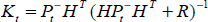
A policy is simply a mapping from beliefs to actions and may be represented as a decision tree over belief ranges. Let us demonstrate this with an example. Imagine a clinic where a patient applies with symptoms of sneezing and fatigue. Dr. John has to diagnose and suspects that the patient suffers from either flu or allergy. For this POMDP problem we have two cases: having flu or having allergy. In order to make the right decision, Dr. John may require tests. After each test, he may require additional tests or may write a prescription. The decision tree of Dr. John is given in Fig. 3 where each ellipse represents an action that is valid for a belief range over having flu given in parenthesis. The top ellipse represents the case when Dr. John's belief that the patient's sickness is flu is between 0.4 and 0.6. For this belief state, Dr. John's decision is to require additional tests.

Fig. 3.

Diagnostic decision tree.

If an n-step policy, π, represented by a decision tree, collects maximum reward in the long term, it is called the optimum policy, π* Each node in the decision tree has a value representing the benefit of choosing the action for that belief range. The benefit calculated by the value function for discrete POMDPs given in Eq. 14 and Eq. 15.

{V_{t}}^{π} (b) = max_{a} Q_{t}^{π} (b, a)

(14)

Where $Q_{t}^{π} (b, a)$ is the value of performing action a at a belief state b at time step t. The calculation of this value is given in Eq. 15.

Q_{t}^{π} (b, a) = E_{π} {\sum_{k = 0}^{n - 1} γ^{k} r_{t + k + 1} ∣ b_{t} = b_{t} = b, a_{t} = a}

(15)

where n is the planning horizon, γ is the discount factor, 0< γ <1.

3. Proposed Approach

In this study, we aim to use POMDP as a model of a real environment in which an agent exists. We further assume that POMDP parameters are not known and that these parameters are continuous. These two assumptions make the problem even harder and such POMDPs cannot be solved exactly.

We use a Kalman filter to calculate Gaussian-based POMDP belief states, under the assumption of A,H,Q and R are time-invariant. This filter returns the best state estimate and its covariance, a measure of uncertainty around the best estimate. The uncertainty gradually converges depending on the measurement, process noise and initial uncertainty value. This feature eliminates the unvisited uncertainty values from value calculation. Moreover, the predictor-corrector algorithm of Kalman filter determines from the current state estimate, the boundaries of the next estimated state at the next uncertainty level for each logically grouped action. Finally, the optimal policy is constructed, which is represented as a finite state automaton (FSA).

3.1. Belief State Representation

Assume a one dimensional maze as shown in Fig. 4. For a discrete POMDP, initially the agent is in either one of the four cells, and the agent's belief can be represented as a vector given in Eq. 16.

b = [0.25 0.25 0.25 0.25]

(16)

Fig. 4.

One-dimensional maze.

In the continuous state case it is impossible to represent each belief as a vector, since there are infinitely many states. So we have assumed the belief as a Gaussian probability distribution where the mean is the most probable current state and the covariance is the state estimation error or uncertainty. Belief formulation at step t is given in Eq. 17, where s_t is the most probable current state and P_t is the covariance.

b_{t} (s) = N (s_{t}, P_{t})

(17)

In the discrete case, the belief state space dimension is one less than the number of states as shown in Fig. 5(a). It is normally expected that for the continuous case since the number of states is infinite, the dimension of the belief state space is also infinite. Using a parametric distribution, i.e. Gaussian, for the belief state representation reduces the infinite dimensions to two dimensions as shown in Fig. 5(b). In our experiments, the initial belief point covariance or uncertainty is P_o = P_max. At the next decision steps Kalman filter decreases the uncertainty level until P_converge. Therefore with 99% probability, the current state is within 2.5×✓P neighborhood of the most probable current state. Although P_converge is always greater than 0 when an observation noise exists, the case where P is equal to 0 is given in the figure since we calculate the reward function from the definition for the MDP case as explained in subsequent sections.

Fig. 5.

One dimensional maze belief state space representations: (a) discrete case (b) continuous case with parametric distribution.

3.2. The Reward Function Calculation

The reward for POMDP problems is always defined for the MDP case. For a MDP, whether discrete or continuous, the reward of taking action a for state s is constant. In the one dimensional maze POMDP problem illustrated in Fig. 4, there exists four discrete states and the goal state is marked with a circle. The reward definition for this problem is +1 for being at the goal state and 0 elsewhere for each possible action. The reward function can be represented by a four dimensional vector [0 0 0 1]. To calculate the reward at belief state [0.25 0.25 0.25 0.25], the vector product of the belief state vector and the reward vector for MDP case is taken which is 0.25 × 0 + 0.25 × 0 + 0.25 × 0 + 0.25 × 1 = 0.25.

The formal definition of reward r(b) for a belief state b is given in Eq. 18, where n is the number of states.

r (b) = \sum_{k = 0}^{n - 1} b_{k} (s) r_{k} (s, a)

(18)

Using this formal discrete definition, to calculate the reward for the belief state N(s, P), we compute an infinite sum of the product of the MDP reward by its probability as shown in Fig 6. Since the reward in MDP case is constant and the state probabilities are represented as Gaussian, this infinite sum is equivalent to the integral in Eq. 19, which is equivalent to cumulative distribution function (cdf) of Gaussian across the range where reward is non-zero. Since with 99% confidence the states lie between 2.5×✓P apart from the most probable state, we have considered only this range as an approximation. In other words we assume the integral bound is s ± 2.5×✓P, where s is the most probable state.

lim_{Δ s \to 0} \sum_{S = - \infty}^{S = \infty} b (s) r_{a} (s) Δ s = \int_{s} b (s) r_{a} (s) d s

(19)

Fig. 6.

The continuous case reward value calculation at a belief state.

To exactly calculate the reward function at some uncertainty level, we need to convolve the MDP reward with all belief points. We suggest a method to approximately calculate the reward function for the continuous case for different uncertainty levels. Since the reward for each action in the MDP case is constant over states, we adjust the edges of the reward function by an approximation. For each edge of the MDP reward, the rewards for the two points 2.5×✓P apart from that edge are computed. Using these two reward values, a new reward function, which is a line passing through these reward values, is generated. The overall reward function for the uncertainty level P is constructed by taking the minimum of the MDP reward and the newly generated lines calculated for each edge where the MDP reward is positive and maximum when the MDP reward is negative.

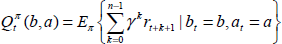
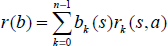
For the continuous case one dimensional maze, the reward function for MDP case and uncertainty level 0.01 is sketched in Fig. 7. Fig. 7(a) is the MDP reward function where the uncertainty is 0. Fig. 7(b) is the newly calculated reward function at the uncertainty level 0.01. Note that for uncertainty 0.01, 2.5×✓P is 0.25, and the edges are approximated. For example, for the edge at location 3, the reward for 2.75 is 0 and the reward for 3.25 is +1. The minimum of generated lines for the edges at 3 and 4, and the MDP reward is shown on Fig. 7(b).

Fig. 7.

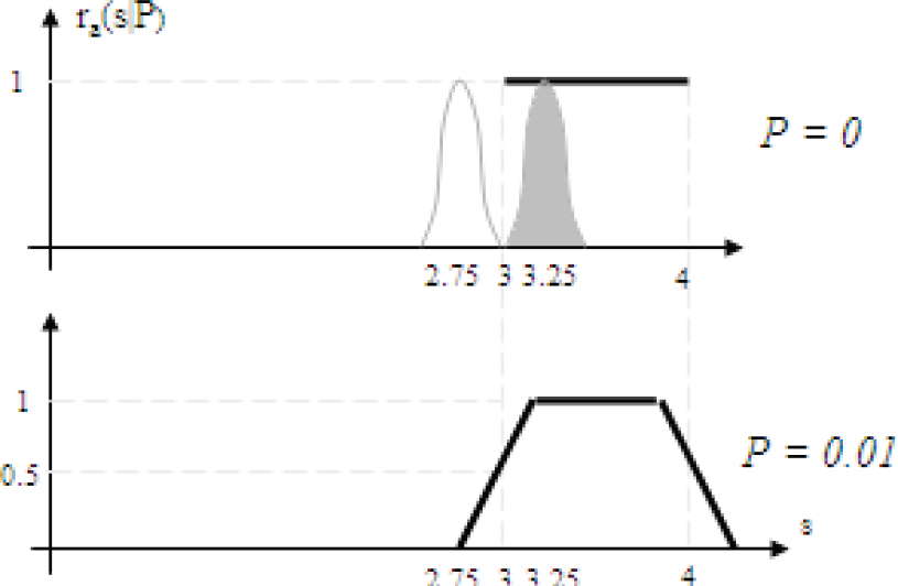
(a) MDP reward function at uncertainty 0. (b) Approximate reward function at uncertainty 0.01.

3.3. Reachable Belief Region Calculation

In this section, we show how to calculate the next step reachable belief points and their weights in continuous case Gaussian-based POMDPs using internal dynamics of the agent and Kalman filter. The final result is a Gaussian probability distribution which represents the weights of reachable belief points as shown in Fig 8. The Kalman filter (Grewal and Andrews 1993, Maybeck 1979) addresses the general problem of trying to estimate the state of the agent. It is governed by stochastic equations Eq. 6 and Eq. 7 Since Kalman filter computes the minimum mean square error estimate of the current state, we use it in the prediction of the next step's reachable belief range calculation. In our experiments, we linearize the systems and use time-invariant parameters for A, H, Q and R. Therefore, at each run the agent starting with the same initial state estimation error, visits same state estimation error values or uncertainty levels. Reachable belief points for a next step all share a common covariance or uncertainty or state estimation error, P_t.

Fig. 8.

Initial belief and the next belief state distribution.

Initial belief state is a Gaussian distribution over states N(s₀, P₀). It can be represented in the belief state space as a single point as shown in Fig. 8. According to the motion model, taking action a₀ disturbed with a Gaussian noise N(0, Q), will result in a Gaussian distribution over a new range of belief states with mean defined by Eq. 20 and the covariance defined by Eq. 21 at the uncertainty level P₁ as shown in Fig. 8 Since the initial belief point is given, at the uncertainty level P₀ then V(s₀) is 0.

E (s_{1 | 0}^{^{-}}) = A E (s_{0}) + B E (a_{0}), s . t . E (s_{0}) = s_{0}

(20)

V (s_{1 | 0}) = A V (s_{0}) A^{T} + B V (a_{0}) B^{T}, s . t . V (s_{0}) = 0

(21)

The state estimation in the prediction phase will be updated in the correction phase depending on the observation. The new mean of the distribution over the next uncertainty level belief states is given in Eq. 22 and the covariance in Eq. 23.

E (s_{1 | 0}) = E (s_{1 | 0}^{^{-}}) + K_{0} (E (o_{0}) - H E (s_{1 | 0}^{^{-}}))

(22)

V (s_{1 | 0}) = V (s_{1 | 0}^{^{-}}) + K_{0} V (o_{0}) - H V (s_{1 | 0}^{^{-}}) H^{T}) K_{0}^{T}

(23)

In POMDP problems like tiger (Cassandra 1999), the observation of the agent is independent of the agent's location. It is dependent on the location of the tiger which is behind one of the doors. Therefore, the possible observations are represented by a Gaussian with mean as the location of the tiger and covariance as the observation noise's covariance. But in navigational type of POMDP problems like one dimensional maze (Cassandra 1999) the observation of the agent is dependent on its location. In the navigational type of POMDP problems, for a given uncertainty level, the observation probability is the convolution of two Gaussian distributions given in Eq. 24

p (o) = \int p (o ∣ s) p (s) d s

(24)

Since the convolution of two Gaussian distributions is also a Gaussian distribution (Bracewell 1999), mean and covariance can be calculated as given in Eq. 25.

\begin{matrix} E (o) = E [0 ∣ s] + E (s) \\ V (o) = V [o ∣ s] + V (s) \end{matrix}

(25)

In navigational type of problems, the observation noise is N(0, R). Consequently, p(o | s) is a Gaussian distribution with mean 0 and covariance R, around s. The reorganized version of Eq. 25 is given in Eq. 26.

\begin{matrix} E (o) = E (s) \\ V (o) = T + V (s) \end{matrix}

(26)

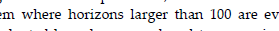
By substituting the mean and the covariance given in Eq. 26 into Eq. 22 and Eq. 23 respectively, we get a Gaussian distribution over the belief states at uncertainty level P₁ for the action a₀ taken at belief state N(s₀, P₀) which represents the probability of next step reachable belief points. Due to the nature of Kalman filter, reachable belief points at the next step all share a common covariance or uncertainty or state estimation error, P_t. The reachable belief points covariance or uncertainty levels can be calculated using Eq. 10, Eq. 11 and Eq. 13. p(s_t+1 | P_t+1) can be calculated recursively from previous step p(st | P_t)using the Eq. 22, Eq. 23 and Eq. 26 as shown in Fig. 9.

Fig. 9.

Final Gaussian showing probability of next step reachable points for one dimensional maze.

To illustrate the idea in one dimensional maze problem, a single Kalman iteration is shown in Fig. 8. A, B and H are modeled as the identity matrix. Let the initial belief be N(s₀, P₀), the observation noise N(0, R), and the actuator noise is N(0, Q). E[aright] is +1 and as expected E[aleft] is −1. Then the next reachable belief points' probability distribution from P₀ to P₁ for aright is N(s₀+1,Q+K²R) computed using the Eq. 22, Eq. 23 and Eq. 26. This result for the next reachable belief points probability distribution complies with the result calculated by convolution of probabilities suggested by Porta, Spaan and Vlassis (Porta et al. 2005) which is $N (s_{0} + E [a], Σ + Σ^{a} + Σ^{o})$ Note that Porta, Spaan and Vlassis calculated the belief state, whereas we calculate the probablity distribution over belief states for a given uncertainty level depending on the possible set of observations and a given action. The slight difference K² which is the coefficient of the observation noise in our calculation is due to Kalman's measurement update equations and since K is a positive number smaller than one, our calculated covariance is always smaller.

3.4. The Horizon N Q-Value Calculation

Let the uncertainty level calculated by the Kalman Filter at time step t be P_t. Using the probability distribution of the next reachable belief points obtained by the methods described in 3.3 and the approximate reward function for each P_t described in section 3.2 the immediate expected reward can be calculated by Eq. 27.

E (r_{t} ∣ P_{t}, a) = \int p (s_{t} ∣ P_{t}) r_{a} (s_{t} ∣ P_{t}) d s

(27)

To compute Eq. 15 for an n step horizon, a tree consisting of all possible actions with depth n should be generated. Each branch in this tree, from root to leaf, represents a policy π. The horizon n Q-value for a policy π is the sum of the rewards for each node in a branch. The optimal horizon n policy is the branch that collects the maximum reward for n steps. For each node the reward is calculated by using Eq. 27 and multiplied with the corresponding discount factor, γ^k where k is the depth of the current node.

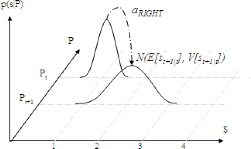
The complete generation of the tree requires O(|A|^N) space and time complexity, where |A| is the number of logically grouped actions and N is the depth or the horizon. To reduce these, we have simply pruned the branches that are never reachable, i.e. beyond world boundaries, and performed a depth first search and kept only the maximum branch ever calculated. The world boundaries are given to the agent as a hint. The boundaries at the uncertainty level are extended by 2.5×✓P_t+k. A sketch of extended boundaries along uncertainty levels for the one dimensional maze is given in Fig. 5. In our experiments, even for the cart pole problem where horizons larger than 100 are evaluated, the evaluated branches are reduced to approximately 2⁸. The space complexity of our algorithm is O(|N|), and the time complexity is O(|A|^d), where d is the average depth of the pruned tree.

For the computation of Eq. 27, since the p(s_t|P_t) is a Gaussian distribution denoted as g(s), and r_a(s_t|P_t) is a linear function denoted as l(s), Eq. 28 contains the product of a Gaussian function g(s) with a linear function l(s);

\int g (s) l (s) d s

(28)

where g(s) and l(s) are given in Eq. 29 and in Eq. 30 respectively.

g (s) = \frac{e^{\frac{- (s - E (s))^{2}}{2 V (s)}}}{\sqrt{2 π V (s)}}

(29)

l (s) = a s + b

(30)

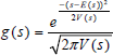
The solution of Eq. 28 is given in Eq. 31 where Φ(s) is the cdf of the Gaussian distribution. Since the approximate reward function for an uncertainty level is piecewise linear, Eq. 31 must be computed separately for each different reward line segment. For example, in Fig. 7 for the reward function computed for uncertainty level 0.01, Eq. 31 is computed for three non-zero reward line segments.

\begin{aligned} \int \frac{e^{\frac{- (s - E (s))^{2}}{2 V (s)}}}{\sqrt{2 π V (s)}} [a s + b] d s = \\ - a \sqrt{\frac{V (s)}{2 π}} e^{\frac{- (s - E (s))^{2}}{2 V (s)}} + [b + \frac{a E (s)}{2 π V (s)}] ϕ (s) \end{aligned}

(31)

3.5. Policy Generation

The Kalman filter equations for the calculation of the state estimation error P only depends on the motion model matrix A, the measurement model H, the process noise Q and measurement noise R and previous state estimation error. In our experiments, we linearize the systems and use time-invariant parameters for A, H, Q and R. Therefore, at each run the agent starting with the same initial state estimation error, visits same state estimation error values or uncertainty levels, but different most probable states, s, as shown in Fig. 10. Moreover, Maybeck (Maybeck 1979) has also shown that the estimation error covariance P of the Kalman filter converges to a unique value from any initial condition where parameters A, H, Q and R are time-invariant. We call this unique value P_converge. Although P_converge can be calculated by solving Ricatti equation, our algorithm decides on convergence if the current value is in the same ∈-interval for last l steps as shown in Fig. 10.

Fig. 10.

Uncertainty levels computed by Kalman Filter.

Constructed policy is represented by a FSA. The internal representation of automaton nodes is as follows:

Uncertainty level label, P_t,

Best action, a,

Belief state, b,

Q-value for a,

N, from which this node is reached.

A set of previous automaton nodes

The transition model of this automaton is deduced by taking the best action from a node. To generate nodes, at each step, the agent decides on a best action by calculating the Q-values as explained in section 3.4. After taking the best action the agent updates its current belief state using Kalman filter, and the new belief state's Q-values and the best action are calculated. In this new belief states' uncertainty level the current belief is compared with the one nearest neighbour (1-NN) node sharing the same uncertainty level if any. If such a point exists and has the same best action than the current belief is not stored. If such a point exists and has some other best action than a new node is generated. Finally, if no such point exists then a new node is generated too.

In our experiments the initial horizon, n is taken a value greater than the step size needed to reach P_converge. Next, all horizons up to m > n are evaluated. If for horizons m-k up to m the number of FSA nodes do not change, we conclude that the policy generation phase is finished where a stable policy is obtained. Finally, we conclude that m-k is the policy convergence horizon for the problem.

4. Experimental Results

The algorithm is run on some well known POMDP problems namely, the tiger problem, the one dimensional maze problem, and the load unload problem. We have run each experiment for horizons 3 to 20. We have also applied our algorithm to the inverted pendulum problem modified as a continuous case POMDP problem for horizons 100 to 180.

4.1 The Tiger Problem

The tiger problem has been converted to continuous observation over discrete states case by Hoey and Poupart (Hoey and Poupart 2005). Although our algorithm works for continuous observation over continuous states, we modeled the tiger problem as defined in (Hoey and Poupart 2005). We assumed that B is equal to the zero matrix, A and H are equal to the identity matrix and only the observation noise exists, N(0, 0.30), i.e., there is no actuator noise. Since the location of the tiger is independent of the agent's location, E(0) in Eq. 25 is equal to either −1 or +1, and V(0) is the observation noise. The penalty of opening the door with the tiger is −100, the reward of opening the door without the tiger is +10 and the cost of listening is −1.

The discount factor is 0.75. Initially E(s₀) is 0, and P₀ is 1. Since the agent may hear the tiger from −1 or +1 disturbed with a Gaussian noise, the agent evaluates listen action for each possible case for each horizon. On the average the agent did not open any doors until the degree of uncertainty, P_n, falls below 0.03 and the estimated location of the tiger is greater than +1.14 or less than −1.22 on the average. Experiments showed that the agent tends to listen for at least 12 steps, in other words, the agent did not open any door for horizons smaller than 13. For horizon 13 or higher the agent opens a door, depending on the uncertainty and the distance of the estimated state from the door locations. Horizon 13 is the policy convergence horizon for this problem. A simple sketch of the resulting FSA is shown on Fig. 11

Fig. 11.

FSA for tiger problem

4.2 The One Dimensional Maze Problem

In the one dimensional maze problem, the goal is placed at the right end. Simulations are done using Webots simulator (Michel 2004). A Webots screenshot is given in Fig. 4.

The agent, can move EAST and WEST or it can STOP. The goal state is marked by a darker color. The agent has a single range finder disturbed with a Gaussian noise. We assumed A, B and H are equal to the identity matrix and the sensor and the actuator is disturbed with noises N(0, 0.45) and N(0, 0.25) respectively.

The discount factor is 0.75. Initially E(s₀) is 0, and P₀ is 0.30. For each horizon the agent preferred moving RIGHT till goal location. P_converge is 0.233. Since the agent begins at zero, it could reach the goal state for horizon five or higher. Horizon five is the policy convergence horizon for this problem. A sketch of the policy FSA is shown on Fig. 12. For uncertainty levels greater than 0 and less than or equal to 0.233, as the uncertainty level increases, the agent will stop closer towards right, in other words the agent stops closer to the right end.

Fig. 12.

FSA for one dimensional maze.

4.3 The Load Unload Problem

In this very challenging problem, the agent acting in a one dimensional maze has a cart that must be driven from an Unload location to a Load location, and then back to Unload. This problem is a simple POMDP with a hidden variable that makes it partially observable (the agent cannot see whether it is loaded or not). If the agent had memory it would remember its latest Load or Unload action, and it would go left or right correspondingly. The agent is a cart designed to shuttle loads back and forth between two end-points on a line of 5 units distance. At the left end we pick up an item from an infinite pile. At the right end, after 4 units, we drop our item. At the left end, before 1 unit, we pick our item. The cart does not have sensors to indicate whether it is loaded or unloaded, but it can determine its position on the line. To act optimally the belief state must encode whether we have an item or not. Actions are simply move WEST, −1 meters, move EAST, +1 unit, LOAD or UNLOAD. Moving in an impossible direction leaves the agent where it is. A reward of +1 is received for picking up when unloaded or putting down when loaded, but only one item can be carried at a time. We assumed H and A are equal to the identity matrix. For actions WEST or EAST, B is the identity matrix, for actions LOAD or UNLOAD, B is zero. The sensor and the actuator are not noisy, so this experiment demonstrates the efficiency of the FSA generation layer only. The discount factor is 0.75. Initially E(s₀) is 0, and P₀ is 0. P_converge is 0.

The resulting FSA is shown on Fig. 13. The policy could reveal the hidden state, whether loaded or unloaded. The previous states kept in FSA provide an implicit memory.

Fig. 13.

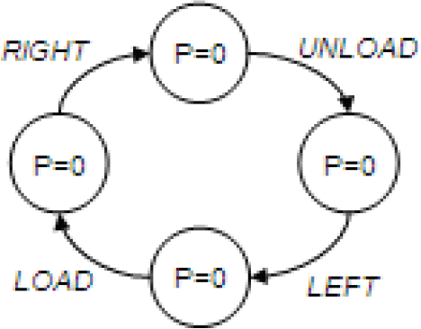
FSA for the load unload problem.

4.4 The Inverted Pendulum Problem

We have applied our algorithm to the well known Cart Pole or Inverted Pendulum Problem. The task is to balance an inverted pendulum hinged to a cart by accelerating and slowing down the cart, as sketched in Fig. 14. If the pole falls the episode ends with a failure and the cart is reset. If the cart moves beyond given limits, the cart is reset with a failure too.

Fig. 14.

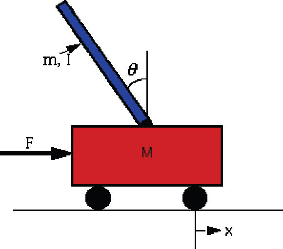
The inverted pendulum problem.

The cart with an inverted pendulum, shown below, is “bumped” with an impulse force, F. We assume that the pendulum does not move more than a few degrees away from the vertical,. For this linearized model, the equilibrium ranges for the pendulum's angle and the cart's position are rewarded by 1, 0 otherwise.

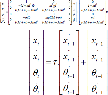
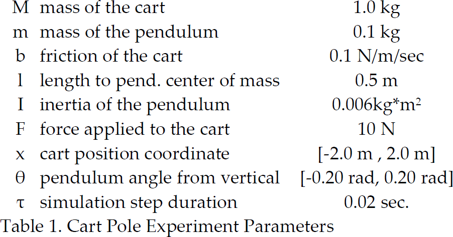
For this experiment, cart pole parameters are given in Table 1. Linearized system equations are given in Eq. 32, and Eq. 33, where mathematical derivations are given in (Math Works 1994).

\begin{aligned} [\begin{matrix} \dot{x} \\ \ddot{x} \\ \dot{ϕ} \\ \ddot{ϕ} \end{matrix}] = [\begin{matrix} 0 & 1 & 0 & 0 \\ 0 & \frac{- (I + m l^{2}) b}{I (M + m) + M m l^{2}} & \frac{m^{2} g l^{2}}{I (M + m) + M m l^{2}} & 0 \\ 0 & 0 & 0 & 1 \\ 0 & \frac{- m l b}{I (M + m) + M m l^{2}} & \frac{m g l (M + m)}{I (M + m) + M m l^{2}} & 0 \end{matrix}] [\begin{matrix} x \\ \dot{x} \\ ϕ \\ \dot{ϕ} \end{matrix}] + [\begin{matrix} 0 \\ \frac{(I + m l^{2})}{I (M + m) + M m l^{2}} \\ 0 \\ \frac{m l}{I (M + m) + M m l^{2}} \end{matrix}] u \\ [\begin{matrix} x_{t} \\ \dot{x_{t}} \\ θ_{t} \\ {\dot{θ}}_{t} \end{matrix}] = τ . [\begin{matrix} \dot{x_{t - 1}} \\ \ddot{x_{t - 1}} \\ \dot{θ_{t - 1}} \\ \ddot{θ_{t - 1}} \end{matrix}] + [\begin{matrix} x_{t - 1} \\ \dot{x_{t - 1}} \\ θ_{t - 1} \\ \dot{θ_{t - 1}} \end{matrix}] \end{aligned}

(33)

Table 1.

Cart Pole Experiment Parameters

M	mass of the cart	1.0 kg
m	mass of the pendulum	0.1 kg
b	friction of the cart	0.1 N/m/sec
1	length to pend, center of mass	0.5 m
I	inertia of the pendulum	0.006kg*m²
F	force applied to the cart	10 N
x	cart position coordinate	[−2.0 m, 2.0 m]
θ	pendulum angle from vertical	[−0.20 rad, 0.20 rad]
τ	simulation step duration	0.02 sec.

The agent's state estimation, $[x, \dot{x}, Φ, \dot{Φ}]$ We can rewrite Eq. 32 and 33 as

\dot{s} (t) = F s (t - 1) + G u (t - 1)

(34)

s (t) = τ \dot{s} (t) + s (t - 1)

(35)

then substituting Eq. 34 in Eq. 35 we get Eq. 36.

s (t) = τ [F + I] s (t - 1) + G u (t - 1)

(36)

Finally we get Kalman filter motion model parameters A and B in Eq. 8 as in equations Eq. 37 and Eq. 38 respectively. H in the sensor model given in Eq. 7 is the identity matrix. Actuator noise is Q˜(0, 0.45) × I, and the sensor noise is R˜(0, 0.05) × I. We assume initial belief uncertainty 5.0 × I, which is quite large meaning that the agent is highly uncertain of its location. The discount factor is 0.75.

A = τ [F + I]

(37)

B = G

(38)

The agent could keep the pole balanced for more than 900,000 steps. The state estimation errors are segmented into three uncertainty levels. For the highest uncertainty level, one node exists, the Q-values for the two actions are similar. The second level has 38 nodes. For the lowest uncertainty level, there are 116 nodes. 171 is the policy convergence horizon.

The pole balancing algorithm has not been modeled before for the noisy observations and noisy actuator. Although a variation of VAPS algorithm has been applied to this problem for the POMDP case (Peshkin et al. 1999), they have assumed that x and θ are completely known or observable and no noise in the external input. Moreover, they have assumed that the world model is known and discretisation over belief state space is given before the experimentation. If history for x and θ are kept, their derivatives may be found, and all state variables will be revealed making the case a fully observable MDP. They have concluded in the same way and kept history revealing all state variables. Instead of dealing with unexpected noise values in each step of simulation, with simplifying assumptions they have solved problem just by keeping history which amounts to a fully observable MDP. They have reached 500,000 steps of iteration without failure.

5. Conclusion

The KBFSC algorithm introduced in this study deals with continuous Gaussian-based POMDPs, and as a new approach suggests making use of Kalman filters. The Kalman filter approach assumes that the motion and sensor models are given and their noise can be modeled as Gaussian. It enables easy pruning of unreachable belief points and provides a method to compute approximately horizon N Q-values. KBFSC also suggests a method to calculate an approximate reward function at each horizon.

Moreover, our algorithm is resistant to dynamically changing environments, where it simply looks ahead, and once it locates itself using a Kalman filter, decides on the best action, using simple mathematical equations. Nearly all previous studies assumed discrete POMDPs. As a comparative work, Porta, Spaan and Vlassis (Porta et al. 2005) suggested a method for Gaussian-based POMDPs with continuous state space and discrete observation space. Alternatively, Hoey and Poupart (Hoey and Poupart 2005) suggested a method for Gaussian-based POMDPs with discrete state space and continuous observation space. Both assume that the world model is given, and use PBVI technique (Pineau et al. 2003)for Gaussian-based POMDPs. They calculated value iteration on a pre-collected set of beliefs, while the Bellman backup operator is analytically computed given the particular value function representation. To collect beliefs, the agent has to make extensive exploration. KBFSC has no need to keep belief points and corresponding α-vectors, in order to calculate the next horizon value function, rather KBFSC keeps only representative belief points. KBFSC can foresee the reachable belief points by the virtue of Kalman filter state estimation techniques, and can calculate the horizon n policy by using simple mathematical equations.

Moreover, KBFSC handles continuous state and observation space, and makes decisions dynamically. Although as in the PBVI the solution is dependent on the initial belief, policy generation by using KBFSC does not keep α-vectors and has no belief point set expansion and pruning phase for α-vectors, rather KBFSC keeps only representative belief points. In summary, KBFSC is time and space efficient, as opposed to point based methods. Moreover, the policy always converges given a sufficiently distant horizon which is problem dependent. In real world applications, motion and sensor noises are rarely constant. For example, when an agent navigates on a carpet, it is normally expected to have a different noise characteristic compared to navigation on a marble floor. Our study assumed that motion and sensor noises are assumed to be constant. As a future work, we plan to adapt the method for dynamically changing noise characteristics.

References

Astrom

K.J.

(1965). Optimal control of Markov decision process with incomplete state estimation. Mathematical Analysis and Applications 10, 174–205.

Boyen

and Koller

(1998). Tractable inference for complex stochastic processes. In: Proceedings of the Conference on Uncertainty in Artificial Intelligence. pp. 33–42.

Bracewell

(1999). Two-Dimensional Convolution. Vol. 1. McGraw-Hill.

Cassandra

(1999). Tony's POMDP File Repository Page. http://www.cs.brown.edu/research/ai/pomdp/examples/index.html.

Grewal

and Andrews

(1993). Kalman Filtering. Prentice Hall.

Hoey

and Poupart

(2005). Solving pomdps with continuous or large discrete observation spaces. In: Proceedings of the Nineteenth International Joint Conference on Artificial Intelligence. IJCAI. Edinburgh, Scotland. pp. 1332–1338.

Howard

R.A.

(1960). Dynamic Programming and Markov Processes. The MIT Press, Cambridge MA.

Kaelbling

L.P.

Littman

M.L.

and Moore

A. P.

(1996). Reinforcement learning: A survey. Journal of Artificial Intelligence Research 4, 237–285.

MathWorks (1994). Example: Modeling an Inverted Pendulum. http://www.library.cmu.edu/ctms/ctms/examples/pend/invpen.htm.

10.

Maybeck

P.S.

(1979). Stochastic models, estimation and control. Academic Press.

11.

Michel

(2004). Cyberbotics ltd - webotstm: Professional mobile robot simulation. International Journal of Advanced Robotic Systems 1, 39–42.

12.

Peshkin

Meuleau

and Kaelbling

L. P.

(1999). Learning policies with external memory. In: Proceedings of the Sixteenth International Conference on Machine Learning ( Bratko

and Dzeroski

, Eds.). Morgan Kaufmann. San Francisco, CA. pp. 307–314.

13.

Pineau

Gordon

and Thrun

(2003). Point-based value iteration: An anytime algorithm for pomdps. In: Proceedings of the Sixteenth International Joint Conference on Artificial Intelligence. IJCAI. Acapulco, Mexico.

14.

Porta

J.M.

Spaan

M.T.J.

and Vlassis

(2005). Robot planning in partially observable continuous domains. In: Robotics: Science and Systems I ( Sukhatme

G. S.

Thrun

and Schaal

, Eds.). MIT Press. pp. 217–224.

15.

Sallans

(2000). Learning factored representations on partially observable markov decision process. In: Neural Information Processing Systems. MIT Press. pp. 1050–1056.

16.

Sondik

E.J.

(1978). The optimal control of partially observable markov processes over the infinite horizon: Discounted costs,. Operations Research 26, 282–304.