Sage Journals: Discover world-class research

Abstract

Speeded-Up Robust Feature (SURF) algorithm is widely used for image feature detecting and matching in computer vision area. Open Computing Language (OpenCL) is a framework for writing programs that execute across heterogeneous platforms consisting of CPUs, GPUs, and other processors. This paper introduces how to implement an open-sourced SURF program, namely OpenSURF, on general purpose GPU by OpenCL, and discusses the optimizations in terms of the thread architectures and memory models in detail. Our final OpenCL implementation of OpenSURF is on average 37% and 64% faster than the OpenCV SURF v2.4.5 CUDA implementation on NVidia's GTX660 and GTX460SE GPUs, repectively. Our OpenCL program achieved real-time performance (>25 Frames Per Second) for almost all the input images with different sizes from 320*240 to 1024*768 on NVidia's GTX660 GPU, NVidia's GTX460SE GPU and AMD's Radeon HD 6850 GPU. Our OpenCL approach on NVidia's GTX660 GPU is more than 22.8 times faster than its original CPU version on Intel's Dual-Core E5400 2.7G on average.

Keywords

OpenCL OpenSURF General Purpose GPU

1. Introduction

As a robust image detecting and describing algorithm, Speeded Up Robust Features (SURF) [1] is widely used in computer vision areas. SURF calculates the descriptors and features in a faster way comparing with other similar algorithms like Scale-invariant feature transform (SIFT) [2], and has a good stability against rotation, scale and changes in lighting condition of the processed images. Among the different approaches of SURF algorithm, OpenSURF is an open-sourced, clean, and unintrusive SURF feature extraction library written in C++ with OpenCV support, and implemented on CPU [3].

Open Computing Language (OpenCL) [4] is an open royalty-free standard for general purpose parallel programming across CPUs, GPUs and other processors, giving software developers portable and efficient access to the power of these heterogeneous processing platforms. It is created by the Khronos Group with the participation of many industry-leading companies and institutions, like Apple, NVidia, Intel, AMD, and QualComm, etc. OpenCL includes a C-like language (based on C99) for writing kernels, which are functions executing on OpenCL devices as parallelized threads, plus APIs that are used to define and then control the platforms. OpenCL provides parallel computing using task-based and data-based parallelism. Comparing with other GPU programming platforms like NVidia CUDA (Compute Unified Device Architecture) and AMD/ATI Stream, OpenCL provides an unified and portable programming interface in a heterogeneous environment. Programs written in OpenCL can run on different graphics cards without any modification.

Some researchers studied how to parallelize SIFT and SURF on multi-core CPUs. For instance, Chen P. et al. [5] introduced how to design and implement an adaptive pipeline parallel scheme (AD-PIPE) for both SIFT and SURF to alleviate these limitations on muitl-core CPUs. So far, most of the GPU implementations of image processing algorithms are written in CUDA. For instance, Wu C. [6] introduced how to implement and optimize the SIFT algorithm on CUDA and NVidia's GPUs. Terriberry B. et al. [7] introduced how to port the SURF algorithm to GPU, and presented a novel optimization to compute the integral images. Cornelis N. et al. [8] also published a GPU implementation of SURF algorithm. Their works mostly focused on the shader program and GPU specific memory usage. Furgale P. et al. [9] first modified the OpenSURF code and implemented another algorithm called CPU-SURF, and then implemented the GPU approach on CUDA. Schulz A. et al. [10] introduced a GPU implementation on CUDA, which has similar interfaces like OpenSURF. Other researchers [11 –13] also presented their works in terms of how to implement and optimize the SURF algorithm on multi-core architectures and GPUs. For OpenCL platforms, Mistry P. et al. [14] introduced how to analyse and profile the components of SURF algorithm, and developed a profiling framework which could be used to identify performance bottlenecks and performance issues on different hardware platforms. They more discussed how to use profiled information to tailor performance improvements of SURF for specified platforms than how to design and implement the OpenCL optimizations. Kayombya P. [15] introduced how to implemented and optimized SIFT on OpenCL and GPU as well, and compared the results with the original SIFT algorithm.

In this paper, we introduce how to implement and optimize the OpenSURF library on OpenCL and General Purpose GPU (GPGPU). We did not simplify or redesign the mathematical operations in the original OpenSURF program, but inheriting all the calculations from CPU-based program, except some OpenCV based functions, which can not be supported by OpenCL directly and have to be redesigned and reimplemented. We introduce the optimizations of kernel functions in details, and demonstrate the performance of the GPU implementations module by module. Our final OpenCL implementation of OpenSURF is on average 37% and 64% faster than the OpenCV SURF CUDA implementation 2.4.5 on NVidia's GTX660 and GTX460SE GPUs, repectively. Our OpenCL program achieved real-time performance (>25 Frames Per Second, FPS) for almost all the input images with different sizes from 320*240 to 1024*768 on NVidia's GTX660 GPU, NVidia's GTX460SE GPU and AMD's Radeon HD 6850 GPU. The OpenCL approach on NVidia's GTX660 GPU is more than 22.8 times faster than its original CPU version on Intel's Dual-Core E5400 2.7G on average, and produced almost the same results of the interest points for the input images. In Section 2, we briefly introduce the difference between CUDA and OpenCL. We present the basic structure of OpenSURF and the runtime hotspots on CPUs in Section 3. We discuss the OpenCL implementations and optimizations in Section 4. At last, in Section 5 and 6, we demonstrate the runtime performance of our OpenCL program on GPUs and CPUs, and conclude our work.

Figure 1.

Thread architectures in CUDA and OpenCL.

2. Difference between CUDA and OpenCL

CUDA is one of the most mature and widely used frameworks in GPGPU programming. CUDA programmers could easily find that OpenCL has many similarities with CUDA. Fig. 1 shows the differences of the thread architectures in CUDA and OpenCL [16]. The left part in Fig. 1 demonstrates the CUDA thread architecture and the right part demonstrates the Open CL's. In CUDA, the grid refers to the set of all the threads that execute the same kernel function. And the grid is organized as arrays of blocks of the same size. A block is assigned to a Streaming Multiprocessor, and further divided into 32-thread units called warps. The size of warps can vary from one implementation to another. For instance, On NVidia's GTX series, each warp consists of 32 threads.

In OpenCL, a NDRange is a N-dimensional index space, where N stands for one, two or three dimensions. The work-group is a coarse-grained decomposition of the index space that is similar to the grid in CUDA. An instance of the executing kernel is called a work-item. It is similar to the thread in CUDA. The thread architectures of both CUDA and OpenCL are similar except that the warp concept is weakened in OpenCL. However, in fact, the warp is still the basic unit in the creation, management, scheduling and execution of threads by multiprocessors in OpenCL. Individual threads composing a warp start together at the same program address but are otherwise free to branch and execute independently. When a multiprocessor is given one or more thread blocks to execute, it splits them into warps that get scheduled by the SIMT unit[17].

Table 1 shows the differences of the memory models between CUDA and OpenCL [16]. In CUDA, local memory is private to each thread. Each thread block has a shared memory visible to all threads in the block and with the same lifetime as the block. All threads will access to the same global memory. The constant and texture memory spaces can also be accessed by all threads. The texture memory has some properties that make it extremely useful for computing. For instance, the texture memory is cached on chip, so in some situations it will provide higher effective bandwidth by reducing memory requests to off-chip DRAM. Specifically, texture caches are designed for graphics applications where memory access patterns exhibit a great deal of spatial locality. OpenCL has almost the same memory model as CUDA, except the texture memory. However, the ImageBuffer in OpenCL has similar characteristics with texture memory in CUDA.

Table 1.

Comparison of memory models between CUDA and OpenCL

CUDA	OpenCL	Readable/Writable

local memory	private memory	R /W
shared memory	local memory	R /W
global memory	global memory	R /W
constant memory	constant memory	Readable
texture memory	image buffer	Readable

Figure 2.

Image processing stages of OpenSURF.

In addition, CUDA uses a static compiler to compile the kernel and host code before launching the program on GPU. While OpenCL uses the ahead-of-time (AOT) or just-in-time (JIT) compiler, which has good portability, but will always include the compilation time in total execution time. Due to the AOT compilation, OpenCL needs to do some additional initializations at runtime, for instance, looking for OpenCL devices and creating context for them, creating the command queue for the context and compiling the kernel source code on-the-fly if necessary, and creating kernel objects for kernel functions, etc.

3. OpenSURF on CPU

OpenSURF processes input images as following logical stages: 1) integral image computation; 2) construction of the scale space,; 3) feature detection; 4) orientation assignment, and 5) calculating feature descriptors, which record the feature points detected by SURF as vectors, like the left part of Fig. 2. Every stage takes the previous one's outputs as inputs. After the last stage, the program will generate the descriptor vectors for the feature points. The right part of Fig. 2 gives the corresponding hotspot functions in OpenSURF library, namely Integral(), buildResponseLayer(), isExtremum(), getOrientation() and getDescriptor(), to the logical stages.

Figure 3.

Input image sample 1 from [6].

Figure 4.

Runtime hotspots of OpenSURF on CPUs.

Fig. 4 demonstrates the runtime hotspots of OpenSURF functions for the input image in Fig. 3 with size 640*480, on Intel's ATOM 1.0G and Dual-Core E5400 2.7G CPUs, respectively. The previous CPU is more like an embedded processor, and the latter one is a typical desktop CPU. The stages of orientation assignment and calculating feature descriptors, i.e. the functions GetOrientation() and GetDescriptor(), dominate most of the total execution time, around 80%, on both CPUs. The stage of integral image computation, i.e. the function integral(), occupies least execution time in hotspots, only around 1%. In general, when we parallelize the sequential CPU modules on GPU, we will pay more attentions to the top hotspots like GetDescriptor(). However, as what we will discuss later, with the increment of parallel degrees of the top hotspots, other functions, even the least hotspots like integral(), could become the new bottlenecks. The “others” parts in Fig. 4 include the I/O time and the execution time of other non-hotspot functions.

4. Parallelize OpenSURF on OpenCL and GPGPU

This section introduces the implementations and optimizations of the five logical stages of OpenSURF on OpenCL and GPGPUs. Although the latter stages take more execution time comparing with the previous ones, like Fig. 4, we will introduce the OpenCL implementations by the processing order for an input image.

Figure 5.

Area computation using integral images.

4.1. Integral image computation

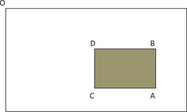
Given an input image I and a point (x, y), the integral image II is calculated by the sum of the values between the point (x, y) and the origin, like Formula 1:

I I (x, y) = \sum_{i = 0}^{i ⩽ x} \sum_{j = 0}^{j ⩽ y} I (x, y)

(1)

Fig. 5 shows that it takes only four lookups and three additions to calculate the sum of the values over any upright, rectangular area after the integral image is computed, like Formula 2:

S = A + D - (B + C)

(2)

In considering the algorithm for computing the integral image on GPU, it can be computed by conducting two passes of prefix sum calculations: first pass along the rows, and then the other along the columns based on the results of the first pass.

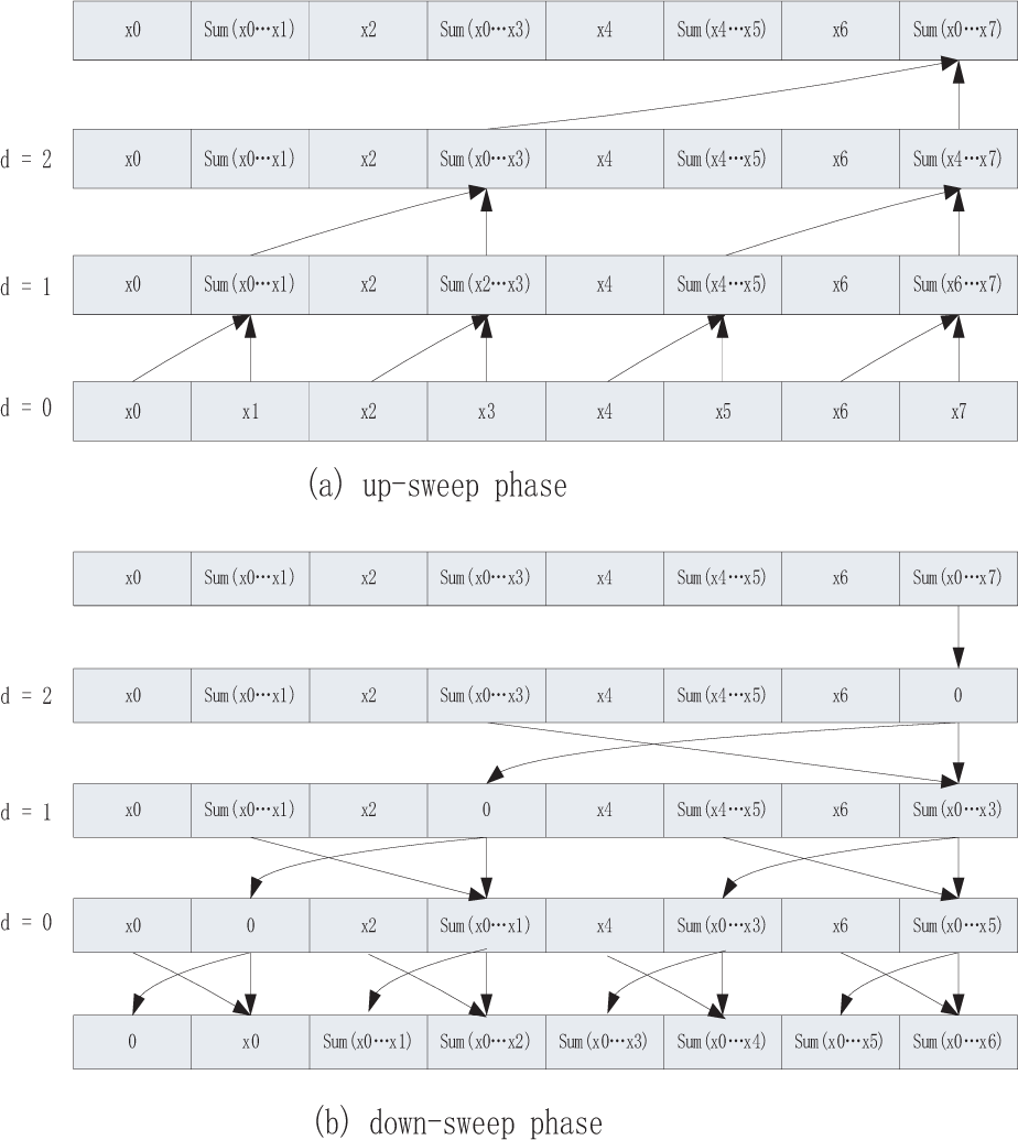
The CUDA Parallel Primitives (CUDPP) library provides methods and interfaces for computing the prefix sums in parallel [18]. However, for OpenCL platform, we have to implement them by ourselves. We use an algorithm similar to the approaches of [19] and [20] to calculate the prefix sums in parallel, like Fig. 6. In the up-sweep and down-sweep phases, we split the prefix sum calculation in multiple steps, with the increment of d from 0 to log₂ n – 1 and decrement from log₂ n – 1 to 0. In each step, we assign different threads to different array items to perform the calculation concurrently, and place synchronizations between every two steps to ensure the data correctness.

We use two GPU kernels to compute the prefix sums along the rows first, then along the columns. In practical, the number of workgroups of the two kernels equal to the size of rows and columns of the image. The number of threads in each workgroup should be configured as a 2-power integer, which should be greater than or equal to the size of columns and rows. For NVidia's GPUs like GTX660 and ION, the maximal number of threads in each group is limited to 512. So, each thread in a workgroup may operate more than one array item, like two, for an input image with size 1024*768. Because the global memory accesses of the second kernel function were mostly non-coalesced and the utilization rate of the memory bandwidth was not high, interchanging the column-scanned values to row-scanned ones before the second GPU kernel start could obviously improve the memory utilization rate.

Figure 6.

The up-sweep and down-sweep phases of parallel prefix sum calculation.

4.2. Constructing the scale space

As a robust local feature detector, the SURF detector is based on the determinant of the Hessian matrix, which is a square matrix of second-order partial derivatives of a function. Given a point x = (x, y) in an image I, the Hessian matrix H(x, σ) at x with σ is defined as Formula 3:

H (x, σ) = [\begin{matrix} L_{x x} (x, σ) & L_{x y} (x, σ) \\ L_{x y} (x, σ) & L_{y y} (x, σ) \end{matrix}]

(3)

Where L_xx(x, σ) is the convolution of the Gaussian second order derivative ∂²g(σ)/∂x² with the image I at point x, and similarly for L_xy(x, σ) [3]. These derivatives are known as Laplacian of Gaussians. Bay [1] proposed an approximation to the Laplacian of Gaussians by using box filter representations of the respective kernels.

In order to detect interest points using the determinant of Hessian, it first needs to introduce the notion of a scale space. The scale space is typically implemented as an image pyramid. The SURF algorithm leaves the original image unchanged and varies only the filter size to construct the scale space. The operations to get the values of Hessian matrix are pixel-independent, and could be calculated in parallel. With the increment of the filter sizes, the number of values need to be computed will decrease. For instance, the filter sizes in OpenSURF could be:

{9, 15, 21, 27, 39, 51, 75, 99, 147, 195}

Figure 7.

Constructing the scale space.

Figure 8.

Example of coalesced access pattern. All threads access the corresponding memory addresses within a segment.

Figure 9.

Example of non-coalesced access pattern. Different threads access different segments.

The numbers of Hessian matrix values needed to be computed will decrease as the following factor array:

{1, 1, 1, 1, 0.5, 0.5, 0.25, 0.25, 0.125, 0.125}

Fig. 7 shows the parallelized computing process of the Hessian matrix. The number of threads relates to the pixel number of the largest layer in the scale space. For instance, if the largest layer in the scale space has 1024 * 768 pixels, we will start (1024/2) * (768/2) = 196608 threads to calculate the scale space in parallel. However, when the sizes of layers decrease, some threads may finish their works before others. For instance, some threads, like thread a in Fig. 7, will run the computing tasks from the first layer to the last one, but other threads, like thread b, may simply return on the half way because of no task left for them in the smaller layers.

When constructing the scale space, the program will intensively access the global memory of GPU, in which the image pyramids are saved. In general, the global memories of GPUs provide higher bandwidths comparing with CPUs, but they also could have extremely high access latencies under some scenarios. For instance, one of the major factors that affect the global memory bandwidth is whether or not accessing the global memory in a coalesced mode. Fig. 8 and Fig. 9 show examples of coalesced and non-coalesced global memory access patterns [21].

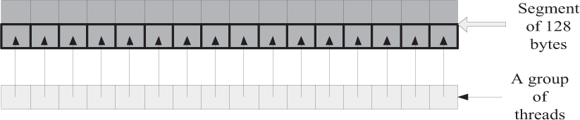
The global memory on GPU is usually divided into segments of 32, 64 and 128 bytes. When accessing a portion of global memory, all threads in the same workgroup should access the same segment of global memory at one time in order to take full advantage of the bus bandwidth. If so, the simultaneous global memory accesses by each thread within a workgroup will be coalesced into a single access, like Fig. 8. Otherwise, the global memory accesses will be conducted to a non-coalesced mode. Under the latter scenario, all the accesses to different segments will be serialized, and will introduce significant memory access overheads.

When constructing the scale spaces, we try to arrange all the global memory accesses in a coalesced mode. For instance, the determinants of Hessian response and Laplacian sign will be calculated by the follow statements in the OpenCL program, like:

\begin{array}{l} r e s p o n s e s [n * h * w + g i d] = (D x x * D y y - 0.81 * D x y * D x y) \\ l a p l a c i a n [n * h * w + g i d] = (D x x + D y y > = 0 ? 1 : 0) \end{array}

In which, the factor n represents the layer of the scale space, h is the half height of the input image, w is the half width of the input image, and gid is the global ID for every thread. Because the numbers of Hessian matrix values will decrease by factors in the aforementioned factor array, the two arrays with the same size of 10 * h * w in the global memory used to store the determinants of Hessian response and Laplacian sign will have some redundancy. The access patterns of global memory for a 1024 * 768 image are shown in Fig. 10.

Figure 10.

The global memory access patterns of all threads when constructing the scale spaces.

The up-left part of Fig. 10 with deeper grey represents the memory space really used and accessed by the threads. About 1/64 of the entire threads will perform the full calculations for all layers, and others will only work for part of the layers, just like Fig. 7.Fig. 10 also shows that the k-th thread will only access the memory at offset k * sizeo f (float) for every working layer, and threads with continuous global IDs will access continuous global memory. Considering the coalesced access pattern presented in Fig. 8, it is to conclude that the access patterns for all threads are coalesced, when the workgroup sizes equal N times of the segment length, e.g. 512.

4.3. Feature detection

At the feature detection stage, SURF first removes the values below the predetermined threshold, and then obtains candidate points by applying a non-maximum suppression (NMS) step in order to extract stable points. At last, the algorithm will interpolate the nearby data on this candidate points [22, 23]. At NMS step, each piece of data in the scale-space will be compared to its 26 neighbours, comprised of the 8 points in the native scale and the 9 points in each of the scales above and below, like Fig. 11.

Figure 11.

Non-maximal suppression.

OpenSURF divides the scale-space into 8 octaves, 3 layers per octaves by default. The feature detection stage will be processed in the middle layers. We parallelize the corresponding GPU kernel function in a way similar to the constructing scale-space kernel function. The thread number equals to the number of pixels that need to be detected on the largest middle layer in the total 8 octaves. The number of values need to be detected in each octave is different, so the GPU threads will process different values independently. When the feature points being found, an atom value will be increased to get the unique index, which will be used to store the feature vectors in a global array for marking.

4.4. Orientation assignment

To assign the orientation for the feature points, we first need to calculate the Haar wavelet responses of size 4s in x and y direction within a circular neighbourhood of radius 6s around the interest point, with s the scale at which the interest point was detected [1]. In mathematics, the Haar wavelet is a sequence of rescaled “square-shaped” functions which together form a wavelet family or basis. The responses are weighted with a Gaussian centred at the interest point. The dominant orientation is selected by rotating a circle segment covering an angle of π/3 around the origin. At each position, the x and y-responses within the segment are summed and used to form a new vector. The longest vector lends its orientation to the interest point [3].

Obviously, we can simply assign a GPU thread to every feature point to calculate its orientation in parallel. Based on this idea, we implement the kernel function called f1 (showed on the left of Fig. 12). Each thread in the kernel will loop 109 times to calculate the Haar responses, because 109 pixels will be used to calculate the Haar wavelet responses within a circular neighbourhood of radius 6s around the interest point.

With a deeper analysis on the original code of OpenSURF, we found that the calculations of Haar wavelet responses were pixel-independent. Therefore, the 109 pixels could be used to calculate the Haar wavelet responses in parallel for every feature point. OpenSURF uses a sliding window with the size π/3 and a step of 0.15, so we can get ⌈2π/0.15⌉ = 42 new vectors per feature. Every vector includes 2 or 3 pixels. With the reference to [10], we reconfigure the feature points as workgroups instead of threads, and assign 42 threads for each workgroup. When threads within a workgroup calculate the Haar wavelet responses for 109 pixels, each thread will work on 2 or 3 pixels with 2 or 3 loops in parallel. All the calculations and the tasks of forming vectors will be processed in local memory. And then we will select the longest vector as the feature's orientation. As the result, we get the improved kernel function called f2 (showed on the right of Fig. 12).

Figure 12.

The control flow chars of kernel functions f1 and f2.

Table 2.

Runtime performance of f1 and f2 on NVidia's GTX260

Image Size	320*240	640*480	800*600	1024*768

f1(ms)	8.09	8.49	9.36	11.75
f2(ms)	0.36	1.36	2.21	3.74

Table 2 presents the runtime performance of f1 and f2 for the input image of Fig. 3 with different sizes on NVidia's GTX260. We can find that f2 is much faster than f1. Some of the reasons are, the number of threads of f2 is much larger than f1, and each thread's computing task of f2 is much simpler than f1. This phenomenon matches the GPU computing principle: the larger number of threads, which have simple computing tasks executing on large amount of process units, could obtain better performance.

4.5. Calculating feature descriptors

When extracting the descriptor, we need to construct a square region centred on the interest point and oriented along the orientation selected in the previous section. The size of window is 20s. Then the descriptor window will be divided into 4*4 regular sub regions. Within each sub region, Haar wavelets will be calculated for 5*5 regularly distributed sample points.

Figure 13.

The flow chart of extracting descriptor vectors in OpenSURF.

If we refer to the x and y wavelet responses by dx and dy respectively, then for these 25 sample points we will collect a vector v = v = {Σdx,Σdy,Σ|dx|,Σ|dy|}. Each sub region contributes four values to the descriptor vector, which will have a length of 4*4*4 = 64 values. At last, the descriptor vector will be normalized [1].

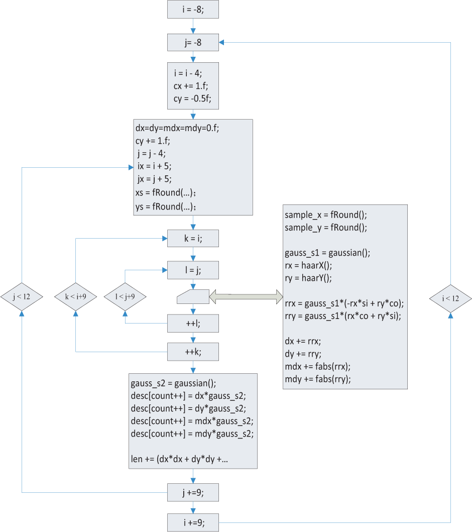
OpenSURF uses 4 loops to compute the feature descriptor vectors, like Fig. 13. The outer two loops that both iterate 4 θ 4 times, corresponding to the 4*4 sub regions, while the inner two loops will both iterate 9*9 times to compute the x and y wavelet responses. At last, the descriptor vector will be normalized.

We design and implement two different approaches to process the aforementioned calculations on GPU, to evaluate the runtime efficiency and parallelism. One approach namely m1 simply rewrites the most inner loop body as the GPU kernel, like the left part of Fig. 14. The kernel function should set the size of workgroups to 16*81, corresponding to the loop counts of total four loops. However, we have to limit the size below 512 with the limitation of the NVidia's thread architecture. We reconfigure the kernel's threads as 16*27 per workgroup, and the number of workgroups equal to the number of feature points. The second kernel function in m1 will normalize all vectors in parallel.

Another approach namely m2 is more complicated. It divides the original program into three kernel functions, like the right part of Fig. 14. The first kernel function corresponds to the outer two loops in Fig. 13. It prepares the data xs and ys used for calculating the Haar wavelets in each sub region. These data will be saved in the global memory. We configure 16 threads per workgroup for the first kernel, and the number of workgroups equal to the number of feature points. For the similar reason introduced in Section 4.2, that the k-th thread accesses the global memory at offset k * sizeo f (float) will ensure the access mode for threads within a workgroup to be coalesced.

Figure 14.

The kernel functions of m1 and m2.

The second kernel function will load the data computed in the first kernel, and calculate the Haar wavelets to generate a vector. It will process the inner two 9 * 9 loops as the original OpenSURF C++ code. We configure 81 threads per workgroup for the second kernel, and the number of workgroups equal to the number of feature points multiplying 16, corresponding to the 4 * 4 sub regions. When we load xs and ys that have been prepared in the first kernel, each thread in the same workgroup just depends on the same xs and ys. Therefore, we can obtain the corresponding xs and ys values by the thread workgroup ID according to the global memory location ID. For example, the first set of threads with global IDs from 0–80 corresponds to the global memory offset 0 * sizeo f (float), which equals to the workgroup ID (the first workgroup) of thread 0–80. The second set of threads with global IDs from 81–161 corresponds to the global memory offset 1 * sizeo f (float). The calculation results of a set of 81 threads will be stored in two different local memory buffers, and will be used to calculate Σdx, Σdy, Σ|dx| and Σ|dy| in the future. At last, the function will get the 64-dimensional descriptor vectors and store them in global memory.

The first and second kernels of m2 process the same calculations as the first kernel of m1, just like Fig. 14, with different thread configurations. Comparing with m1, the computing task of each thread in the second kernel of m2 will be three times smaller than the corresponding part of the first kernel of m1, when calculating Haar wavelets in each sub region.

The last kernel function of m2 will also normalize all vectors in parallel, just like the last kernel of m1.

Table 3.

Runtime performance of approaches m1 and m2 on NVidia's GTX260

Image Size	320*240	640*480	800*600	1024*768

m1(ms)	1.86	11.93	24.12	45.59
m2(ms)	1.85	8.08	14.24	25.89

Table 3 shows the time costs of m1 and m2 when processing the input image in Fig. 3 with different sizes on NVidia's GTX260. Although the two approaches have similar performance for the input image with size 320 * 240, m2 is much faster than m1 when the input image sizes growing.

Table 5 could explain why m2 is faster than m1. It shows the runtime performance of the 3 kernels of approach m2, namely K1 – K3, on NVidia's GTX260 for the input image in Fig. 3. We can find that the second kernel dominates most of the execution time of the whole stage, e.g. more than 95%, for all input samples. Because m2 starts three times as many threads for the second kernel K2 as the corresponding part of the first kernel of m1, it is easy to understand that m2 will get much better runtime performance in most cases, although m2 has to pay more global memory access overheads among more kernels.

5. Performance Results

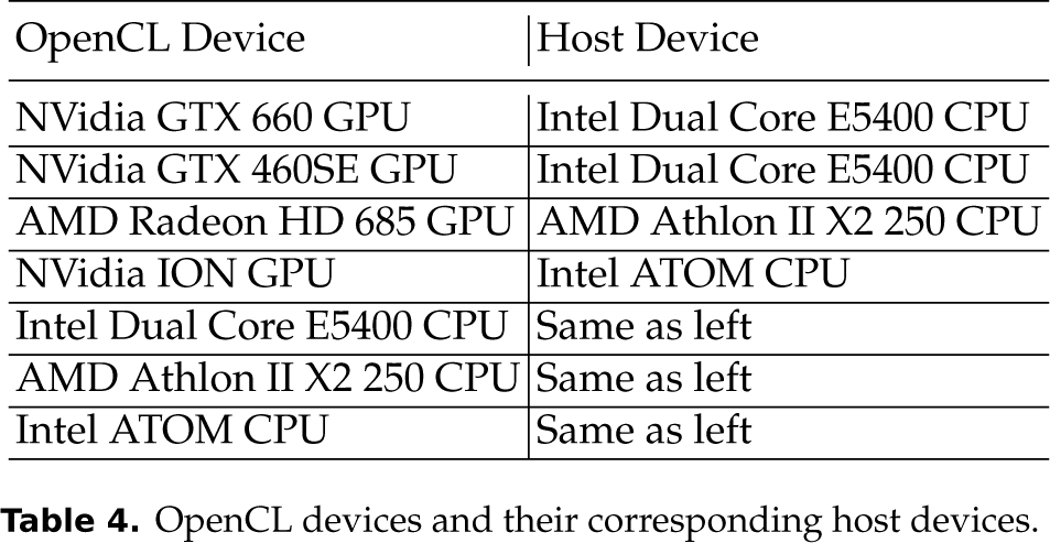
We use 4 different GPUs, i.e. NVidia's GTX660 with 2G on-board GPU memory, NVidia's GTX460SE with 1G on-board GPU memory, AMD's Radeon HD 6850 with 1G on-board GPU memory, and NVidia's ION with 512M shared memory, to evaluate the runtime performance of our OpenCL program. Their host CPUs are Intel's Dual Core E5400 2.7G with 2G main memory for both NVidia's GTX660 and GTX460 GPUs, AMD's Athlon II X2 250 3.0G with 2G main memory for AMD's Radeon GPU, and Intel's ATOM 1.0G with 2G main memory for NVidia's ION GPU, respectively. With the support of AMD APP OpenCL runtime platforms, they are used to be OpenCL devices as well. Table 4 shows the OpenCL devices and their corresponding host devices. The NVidia's OpenCL devices in Table 4 use NVidia's OpenCL v1.1 and CUDA 4.2.9 as the OpenCL runtime platforms. The AMD's Radeon HD 685 GPU and all the OpenCL CPU devices in Table 4, including Intel's Dual Core E5400 CPU, AMD's Athlon II X2 250 CPU and Intel ATOM CPU, use AMD APP SDK 2.7 as the OpenCL runtime platforms. All the host devices are installed an Ubuntu 12.04.2 LTS Linux OS. The version of OpenSURF C++ program is Build 12/04/2012. The OpenCV SURF CUDA implementation used for performance comparison is v2.4.5 that was released on 11/04/2013.

Table 4.

OpenCL devices and their corresponding host devices.

OpenCL Device	Host Device
NVidia GTX 660 GPU	Intel Dual Core E5400 CPU
NVidia GTX 460SE GPU	Intel Dual Core E5400 CPU
AMD Radeon HD 685 GPU	AMD Athlon II X2 250 CPU
NVidia ION GPU	Intel ATOM CPU
Intel Dual Core E5400 CPU	Same as left
AMD Athlon II X2 250 CPU	Same as left
Intel ATOM CPU	Same as left

Table 5.

Runtime performance of 3 kernels of m2 on NVidia's GTX260

Image Size	320*240	640*480	800*600	1024*768

K1(ms)	0.021	0.032	0.041	0.056
K2(ms)	1.810	8.004	14.14	25.75
K3(ms)	0.023	0.045	0.06	0.088

Figure 15.

Input image sample 2 & 3 from [3].

Table 6.

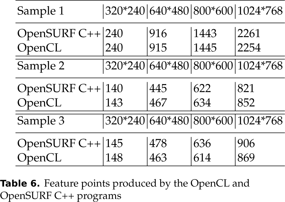
Feature points produced by the OpenCL and OpenSURF C++ programs

Sample 1	320*240	640*480	800*600	1024*768
OpenSURF C++ OpenCL	240 240	916 915	1443 1445	2261 2254
Sample 2	320*240	640*480	800*600	1024*768
OpenSURF C++ OpenCL	140 143	445 467	622 634	821 852
Sample 3	320*240	640*480	800*600	1024*768
OpenSURF C++ OpenCL	145 148	478 463	636 614	906 869

Besides the input image in Fig. 3, we use other 2 images randomly selected from OpenSURF released package in Fig. 15 to evaluate the performance as well.

Table 6 shows the feature point numbers produced by our OpenCL program and the original OpenSURF C++ program for all input images with different sizes. The OpenCL program produces identical feature points on all OpenCL devices we used, and on average more than 95% same as the C program, in terms of both feature point numbers and vectors. Because the OpenCL program calculates the float points in different sequences and different ways comparing with the C++ program, the mathematical results of float points by the two programs could not be always equivalent, but all acceptable in most cases. More about the floating-point errors and how to reduce these errors on GPUs could be found in [24].

Fig. 16 and Fig. 17 present the runtime performance of our OpenCL program on all OpenCL devices in Table 4, the original OpenSURF C++ program on all corresponding host devices, and the OpenCV SURF CUDA implementation v2.4.5 on NVidia's GTX660 GPU and NVidia's GTX460SE GPU, for the 3 input image samples in Fig. 3 and Fig. 15 with different sizes. Our OpenCL program achieved real-time performance (>25 FPS) for almost all sizes of the input images on NVidia's GTX660 GPU, NVidia's GTX460SE GPU and AMD's Radeon HD 6850 GPU, except the first sample with size 1024*267 on NVidia's 460SE (21.8 FPS). For NVidia's GTX660 GPU, NVidia's GTX460 GPU, AMD's Radeon HD 6850 GPU and NVidia's ION GPU, it is on average about 22.8 times, 19.4 times, 20.4 times and 6.9 times faster than the original OpenSURF C++ code on the corresponding host devices in Table 4, respectively. Our OpenCL approach is also on average about 37% and 64% faster than the OpenCV SURF CUDA implementation v2.4.5 on NVidia's GTX660 and NVidia's GTX460SE GPUs. In fact, our approach is faster than the OpenCV SURF CUDA implementation for all input image samples with all sizes, and at most 1.91 times faster for the second sample with size 1024*768 on NVidia's GTX460SE GPU and at least 1.13 times faster for the first sample with size 320*240 on NVidia's GTX660 GPU. We did not compare the performance of our OpenCL program with the OpenCV SURF CUDA implementation on ION, which is more like an embedded hardware platform with much less shared instead of on-board GPU memory comparing with other GPUs, because the OpenCV program always crashed due to insufficient memory errors at the initial stage.

Figure 16.

Runtime performance of our OpenCL program on all OpenCL GPU devices in Table 4, and the OpenCV SURF CUDA implementation v2.4.5 on NVidia's GTX660 and NVidia's GTX460SE GPUs, for the 3 input image samples in Fig. 3 and Fig. 15 with different sizes.

Figure 17.

Runtime performance of our OpenCL program on all OpenCL CPU devices in Table 4, and the original OpenSURF C++ program on all corresponding host CPU devices, for the 3 input image samples in Fig. 3 and Fig. 15 with different sizes.

We tested our program on the OpenCL CPU devices in Table 4 as well, like Fig. 17. It is on average about 1.7 times, 1.29 times and 1.09 times faster than the OpenSURF C++ code on Intel's Dual Core E5400 C2.7G CPU, AMD's Athlon II X2 250 3.0G CPU and Intel's ATOM 1.0G CPU, for the 3 input images with 4 different sizes, respectively. Because all the OpenCL CPU devices only have 2 cores, the speedup numbers are all reasonable. When comparing the performance of our OpenCL approach on CPUs with the OpenSURF C++ code, we turned off the parallelization for the first stage of integral image computation, because the parallelized approach could obviously slow down the performance.

From Fig. 16 and Fig. 17, we can find that the feature point numbers significantly influence the runtime performance for both the OpenCL and C++ programs. For instance, the OpenCL and C++ programs are obviously slower when processing the first sample image than the other two sample images, while the feature points of the first sample image are much more than the other two samples, like Table 6. One reason is, our OpenCL program parallelizes the last stage of calculating feature descriptors depending on the number of feature points. That means, the more feature points we will get, the more threads we will start, just like Section 4.5 introduced. The other reason is, the stage of calculating feature descriptors dominates most of the total execution time for both OpenCL and C++ programs, like Fig. 4 and Fig. 18.

Figure 18.

Speedup of the five stages and the total execution time on OpenCL GPU devices in Table 4 comparing with their corresponding host devices, for a 640*480 input image in Fig. 3. Stages I-V stand for I)Integral, II)Scale space, III)Feature detection, IV)Orientation assignment and V)Feature descriptors, respectively.

Figure 19.

Speedup of the five stages and the total execution time on OpenCL CPU devices in Table 4 comparing with their corresponding host devices, for a 640*480 input image in Fig. 3. The parallelization for Stage I has been turned off for the OpenCL CPU devices.

Fig. 18 shows the speedup of the five stages and the whole program on all OpenCL GPU devices in Table 4 comparing with their corresponding host devices, for a 640*480 input image in Fig. 3. The average speedup numbers of the five stages are 2.22, 56.48, 40.13, 38.34 and 39.92 on NVidia's GTX660 GPU, NVidia's GTX460SE GPU and AMD's Radeon HD 6850 GPU, respectively. Although the first stage is slower on ION comparing with ATOM, the speedup numbers of the whole program are 27.35, 21.56, 24.19 and 7.28 on the 4 different GPUs, repectively.

Figure 20.

Runtime hotspots of the OpenCL program running on OpenCL devices in Table 4 and the OpenSURF C++ program running on the corresponding host devices, for a 640*480 input image in Fig. 3. “Others” stands for the routines not belonging to the five stages, e.g. I/O and helper functions.

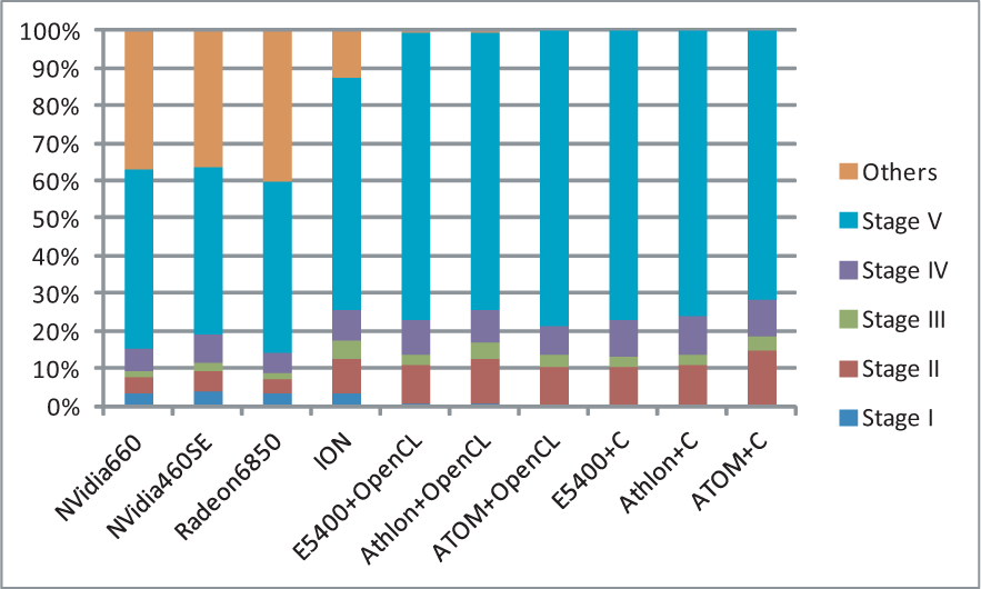
Fig. 19 shows the speedup of the last four stages and the total execution time on all OpenCL CPU devices in Table 4, comparing with the OpenSURF C++ program, for a 640*480 input image in Fig. 3. The parallelization for Stage I has been turned off when computing the total execution time on the OpenCL CPU devices. For the CPUs with OpenCL support, the average speedup times of Stage II-V are 1.41, 1.28, 1.54 and 1.35, respectively, while the first stage could be much slower than the C++ code, e.g. more than dozens of times slower on Intel's Dual Core E5400 C2.7G CPU. From Fig. 18 and Fig. 19, we can also find that the Stage II always get the most speedup times on GPUs comparing with other stages, e.g. more than 66 times faster on NVidia's GTX660 GPU comparing with Intel's Dual Core E5400 CPU, while Stage IV has better speedup performance on OpenCL CPU devices, e.g. more than 1.71 times faster on Intel's Dual Core E5400. That means, the same OpenCL approach may have significant different runtime behaviours on different types of OpenCL devices, especially for GPUs and CPUs. For our OpenCL program, the parallelized approach of the first stage is more suitable for GPUs with dozens even hundreds of cores instead of multi-core CPUs and low-end GPUs with fewer cores like ION. Obviously, although OpenCL programs could run on different types of architectures, the optimizations could be invalid even harmful for some particular devices, while they helps the runtime performance a lot on others. We still need to tune the performance case by case.

Fig. 20 presents the runtime hotspots of the OpenCL program running on OpenCL devices in Table 4 and the OpenSURF C++ program running on the corresponding host devices, for a 640*480 input image in Fig. 3. From Fig. 20, we can find that the OpenCL program running on OpenCL CPU devices has similar hotspot behaviours comparing with the original C++ code, e.g. Stage V of calculating feature descriptors dominating most of the total execution time, while the “Others” parts, including the unparallelized routines like I/O and helper functions, occupy much more percentages of the total execution time on OpenCL GPU devices. It is easy to understand that the unparallelized parts of the OpenCL program might dominate the execution time, when the parallelized stages have been significantly accelerated by GPUs.

6. Conclusion

This paper introduces how to implement and optimize the OpenSURF program on OpenCL and GPGPUs, and presents the kernel functions with the corresponding stages of SURF algorithm in detail. Our experiments show, designing proper thread architectures and memory models for the kernel functions could obviously help the runtime performance. For instance, it is important to configure large number of threads to finish simple computing task for improving performance, especially for platforms with many processing units like GPUs. Because GPUs have different memory models comparing with CPUs, programmers should pay more attention to the global memory access patterns to avoid non-coalesced visits. Out experiments also show, although OpenCL programs could run on different types of architectures, the optimizations could be invalid even harmful for some particular devices, while they helps the runtime performance a lot on others. We still need to tune the performance case by case. The OpenCL and GPU implementation based on this paper has significant performance improvement comparing with the original CPU version.

Footnotes

12. Acknowledgements

This work is supported by the National Natural Science Foundation of China No.61073010 and No.61272166, National Science and Technology Major Project of China No.2012ZX01039-004, and the State Key Laboratory of Software Development Environment of China No. SKLSDE-2012ZX-02.

References

Bay

Tuytelaars

Gool

L.V.

Surf: Speeded up robust features. European Conference on Computer Vision, 1:404–417, 2006.

Lowe

D.G.

Object recognition from local scale-invariant features. Proceedings of the International Conference on Computer Vision. 2.pp.1150–1157. doi:10.1109/ICCV.1999.7904, 1999.

Evans

OpenSURF - Open Source SURF feature extraction library. http://code.google.com/p/opensurf1/.

Munshi

The OpenCL Specification version1.1. Khronos OpenCL Working Group. pages 12–13, http://www.khronos.org/registry/cl/specs/opencl-1.1.pdf.

Chen

Yang

D.L.

Zhang

W.H.

Zang

B.Y.

Chen

H.B.

Adaptive Pipeline Parallelism for Image Feature Extraction Algorithms, Parallel Processing (ICPP), 2012 41st International Conference on, vol., no., pp.299,308, 10–13 Sept. 2012.

SiftGPU: A GPU implementation of scale invariant feature transform (SIFT). http://cs.unc.edu/$cwu/siftgpu, 2007.

Terriberry

T.B.

French

L.M.

Helmsen

GPU accelerating speeded-up robust features. In Proceedings of the 4th International Symposium on 3D Data Processing, Visualization and Transmission(3DPVT′08), pages 355–362, Atlanta, Georgia, June 2008.

Cornelis

Gool

L.V.

Fast scale invariant feature detection and matching on programmable graphics hardware. Proceedings of Computer Vision and Pattern Recognition Workshops, 2008. CVPRW ′08. pages 1–8, June 2008.

Furgale

Tong

C.H.

Kenway

Gaetan

. Gpusurf: Speeded Up Speeded Up Robust Features, http://asrl.utias.utoronto.ca/code/gpusurf/.

10.

Schulz

Jung

Hartte

CUDA SURF: A real-time implementation for SURF, http://www.d2.mpi-inf.mpg.de/surf?q=surf, 2011.

11.

Kim

Park

Chi

Kim

Gruver

W.A.

, A Fast Feature Extraction in Object Recognition Using Parallel processing on CPU and GPU, Proceedings of the 2009 IEEE International Conference on Systems, Man, and Cybernetics, San Antonio, TX, USA, October 2009.

12.

Xie

Gao

Zhang

Liu

, GPU-BASED FAST SCALE INVARIANT INTEREST POINT DETECTOR, Proceedings of Acoustics Speech and Signal Processing (ICASSP) 2010, Dallas, TX, USA, 2010.

13.

Huang

Yan

Chen

, A New Scale Invariant Feature Detector and Modified SURF Descriptor, Proceedings of Sixth International Conference on Natural Computation (ICNC 2010), Yantai, Shandong, China, 2010.

14.

Mistry

Perhaad

Gregg

Chris

Rubin

Norman

Kaeli

David

Hazelwood

Kim

, Analyzing program flow within a many-kernel OpenCL application. In Proceedings of the Fourth Workshop on General Purpose Processing on Graphics Processing Units (GPGPU-4). ACM, New York, NY, USA, 2011.

15.

Kayombya

Richard

, SIFT implementation and optimization using OpenCL, Final Project Report 6.869/6.338, http://beowulf.lcs.mit.edu/18.337–2010/projects/reports/Kayombya_report.pdf, 2010.

16.

Komatsu

Sato

Arai

Koyama

Takizawa

Kobayashi

, Evaluating performance and portability of OpenCL programs, in Proceedings of 9th. International Meeting of High Performance Computing for Computational Science (VecPar 2010), Berkeley, CA, USA, June, 2010.[17]

17.

NVidia, NVIDIA OpenCL Programming Guide for the CUDA Architecture version 2.3, NVidia Inc., 2009.

18.

CUDPP Document, http://www.gpgpu.org/static/developer/cudpp/rel/cudpp_1.1/html/index.html.

19.

Sengupta

Harris

Zhang

Owens

J.D.

, Scan Primitives for GPU Computing, Proceedings of Graphics Hardware 2007, San Diego, California, August 04 – 05, 2007.

20.

Ladner

R.E.

Fischer

M.J.

, Parallel Prefix Computation, Journal of the ACM, Vol 27, No 4, October 1980, pp 831–838.

21.

Yan

Shi

X.H.

Sun

Q.Y.

, An OpenCL Micro-Benchmark Suite for GPUs and CPUs, in Proceedings of the 13th International Conference on Parallel and Distributed Computing, Applications and Technologies (PDCAT′12), Beijing, China, 2012.

22.

Lindeberg

, Feature detection with automatic scale selection, International Journal of Computer Vision, 30(2):79–116, 1998.

23.

Mikolajczyk

Schmid

, An affine invariant interestpoint detector, Proceeding of European Conference on Computer Vision 2002, Copenhagen, Denmark, 2002.

24.

Shi

Wang

, Computing prestack Kirchhoff time migration on general purpose GPU, Computers & Geosciences, 37(10):1702–1710, 2011.

Computing OpenSURF on OpenCL and General Purpose GPU

Abstract

Keywords

1. Introduction

2. Difference between CUDA and OpenCL

3. OpenSURF on CPU

4. Parallelize OpenSURF on OpenCL and GPGPU

4.1. Integral image computation

4.2. Constructing the scale space

4.3. Feature detection

4.4. Orientation assignment

4.5. Calculating feature descriptors

5. Performance Results

6. Conclusion

Footnotes

12. Acknowledgements

References