Sage Journals: Discover world-class research

Abstract

In this paper, we propose a new learning strategy for a probabilistic roadmap (PRM) algorithm. The proposed strategy is based on reducing the dispersion of the generated set of samples. We defined a forbidden range around each selected sample and ignored this region in further sampling. The resultant planner, called low dispersion-PRM, is an effective multi-query sampling-based planner that is able to solve motion planning queries with smaller graphs. Simulation results indicated that the proposed planner improved the performance of the original PRM and other low-dispersion variants of PRM. Furthermore, the proposed planner is able to solve difficult motion planning instances, including narrow passages and bug traps, which represent particularly difficult tasks for classic sampling-based algorithms. For measuring the uniformity of the generated samples, a new algorithm was created to measure the dispersion of a set of samples based on a predetermined resolution.

Keywords

Probabilistic Roadmaps Sampling-Based Motion Panning Dispersion Multi-Query Planner

1. Introduction

A major problem in the development of autonomous robots is in creating a way to give them the ability to make their own motion plans in a variety of situations. Motion planning is the computational process of moving from one initial position to a goal place in the presence of obstacles. A simple version of the motion planning problem is planning a path for a robot between two initial and goal configurations without any collision with present obstacles. This instance of the problem has been shown to be PSPACE-complete. For more complex problems, it is not clear whether the case is even decidable, except for some specific problems [1].

Originally, offline motion planning algorithms required an explicit representation of the configuration space that is a costly and time-consuming procedure for most problems. Sampling-based motion planning was introduced to solve planning queries without attempting to explicitly construct the boundaries of the configuration space. Instead, they rely on a procedure that is able to decide whether or not a given configuration of the robot is in collision with obstacles. There are two main groups of sampling-based path planning methods, namely, roadmap-based or multi-query algorithms and tree-based or single query algorithms [2].

Roadmap-based methods are typically used for multi-query purposes, as they maintain a roadmap that can be used to answer different planning queries. The main data structure used is a graph whose nodes are points in the configuration space. Edges in this graph exist between configurations that are close to one another, and the robot can move from one point to the other without collision. A typical algorithm has two phases: a learning phase and a querying phase. In the learning phase, the roadmap is created. Collision-free configurations, called ‘samples’, are generated randomly and these are the vertices of the roadmap. In the query phase, a number of attempts are made to connect each sample to its nearest neighbours, thus adding edges to the roadmap. To solve a particular query, the initial and goal configurations are added to the roadmap and a graph search algorithm is used to find a path. The efficiency of the algorithm depends on how well the roadmap can capture the connectivity of the configuration space [3]. Moreover, the main performance bottleneck is the construction of the roadmap, since graph search algorithms are fast. One of the most important challenges of this method lies in how to sample useful configurations that will increase the coverage of the roadmap.

In many cases, quickly solving one particular planning problem instance is of interest. For these cases, single query planners can be used. In these planners, the main data structure is typically a tree. The basic idea is that an initial sample (the starting configuration) is the root of the tree and newly produced samples are then connected to samples already existing in the tree. The rapidly exploring random trees (RRT) algorithm [4] is one of the first and most important tree-based planners, and other tree planners are usually an extension of the RRT algorithm. Figure 1 shows the performance of PRM and RRT Algorithms in a 2D indoor environment.

Figure 1.

The performances of two sampling-based planners in a 2D indoor environment. Initial and goal configurations are illustrated by yellow and green squares respectively.

As mentioned before, one of the critical issues in a sampling-based algorithm is the sampling strategy, which can be defined as the procedure of randomly selecting new configurations and adding them to the set of chosen nodes, i.e., a roadmap or a tree. Improving the sampling process is one of the most important aspects in ameliorating the performance of a sampling-based planner. Perhaps the easiest way is to increase the number of samples in the roadmap, which helps the planner to capture the overall connectivity of the configuration space. Unfortunately, augmenting the size of the sample's population will dramatically increase the runtime of the planner. Capturing the connectivity of the workspace and the runtime of the planner are two inconsistent and conflicting concepts, such that any attempt to improve one of them may result in the worsening of the other.

There are several ways of improving the sampling strategy. Some of the previous proposals were based on using the available information of the environment to elucidate the important regions of the configuration space and biasing the sampling in those areas. Randomized bridge builders (RBBs) [5], Gaussian samplers [6] and workspace importance sampling (WIS) [7] are some instances of this type of improvement. In these approaches, the density of the sampling around difficult regions of the workspace is increased. Another way is to use a hybrid adaptive strategy for the sampling. For instance, a hybrid PRM was proposed in [8] that employs different sampling strategies based on the sampling region. Another idea has been to apply several sampling strategies in a chain-like manner [9], starting with a uniform strategy that is followed by other types of sampling strategies. Each of the successive strategies takes its former sampling's results and produces a random output.

A number of deterministic or quasi-random alternatives to pseudo-random strategies have been used in the literature. These alternatives were first introduced in the context of Monte Carlo integration and seek to optimize various properties of the sampling distribution. Before describing the proposed planner, we should discuss some of the mathematical notions for measuring the uniformity of a set of samples. Uniformity can be defined as how well the samples cover the workspace without clumping or gaps. This can be determined in terms of discrepancy or dispersion. A complete overview of these criteria can be found in [10]. Here, we briefly introduce only the concepts needed for this paper. Let Q = [0, Q_x) × [0, Q_y) ⊂ = ℝ² be the space over which to generate samples. The uniformity can be assessed with respect to a specific collection of subsets of Q, called a range space, denoted by R_s. Let R ∊ R_s be one of these subsets. R_s can be the set of all axis-aligned rectangles, the set of all balls or the set of all convex subsets. S is the set of generated samples.

Considering L(R) as the Lebesgue measure (or volume) for R, one can conclude that if the samples in S are ideally uniform, then it seems reasonable that the number of those samples that lie in any subset R should be roughly L(R)/L(Q). The discrepancy is defined to measure how far from the ideal the samples in S are:

D (S, Q) = \sup_{R \in R_{s}} |\frac{|S \cap R|}{N} - \frac{L (R)}{L (Q)}|

[1]

where |A| denotes the cardinality of a finite set A. While, discrepancy - as a measure-based criterion - provides a measure of how uniformly the samples are distributed over the space Q, a metric-based criterion, known as dispersion, provides a measure of the largest portion of Q that contains no samples in S:

δ (S, Q) = \sup_{q \in Q} \underset{s \in S}{m i n} d (q, s)

[2]

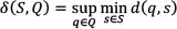
Note that d denotes any metric, such as Euclidean distance.

Intuitively, δ corresponds to the radius of the largest empty ball centres inside the space Q. Therefore, an experimental way to measure the dispersion of a set of samples is to find the largest ball centered in the workspace and containing no samples. We use this method to measure the dispersion of samples resulting from the original PRM and the proposed planner. For measuring the dispersion of a set of samples, we designed a resolution-based algorithm that measures the dispersion value according to any desired resolution. Algorithm 1 presents the pseudo-code of this procedure. This algorithm measures the distance between all points inside the workspace and the closest sample. After finding this value for all points of the configuration space based on a given resolution, the algorithm finds the largest value among them. The largest distance is the dispersion value for the considered set of samples.

Algorithm 1.

Measuring the dispersion of a set of samples.

It was reported in the literature that using a deterministic set of samples instead of random samples outperforms the original PRM [11]. One of the earliest proposals was to use a Halton sequence [11], which generalizes the Van Der Corput sequence to d dimensions. For a 1D sample space S = [0,1], the Van Der Corput sequence gives a set of samples that minimizes both discrepancy and dispersion. The n^th sample in this sequence is generated as follows. Let a_i ∊ {0,1} be the coefficients that define the binary representation of n:

n = \sum_{j} {2^{j} a}_{j} = a_{0} + {2 a}_{1} + {2^{2} a}_{2} + \dots

[3]

The n^th element of the Van Der Corput sequence, Φ(n) is defined as:

Φ (n) = \sum_{j} {2^{- (j + 1)} a}_{j} = {2^{- 1} a}_{0} + {2^{- 2} a}_{1} + \dots

[4]

The Halton sequence is a multi-dimensional variant of the Van Der Corput sequence, and can be defined as follows. Let {b_i} define a set of d relatively prime integers, {2, 3, 5, 7,…, n}, the integer n has a representation in base b_i given by:

n = \sum_{j} a_{i j} b_{j}^{i}, a_{i j} = \{0,1, \dots, b_{j} - 1\}

[5]

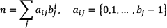
Then, the Halton sequence can be formulated as:

Φ_{b_{j}} (n) = \sum a_{i j} b_{j}^{- (i + 1)}

[6]

The n^th sample is then defined by the coordinates P_n = (Φ_b1(n),Φ_b2(n),…,Φ_bd(n)).

The Halton sequence was applied to the PRM planner (QRM) [12] with proven advantages.

When the number of samples is specified, a Hammersley sequence achieves the best possible asymptotic discrepancy. The n^th point in a Hammersley sequence is obtained by using the first (d − 1) coordinates of a point in the Halton sequence with the ratio n/N as the first coordinate:

P_{n} = (\frac{n}{N}, Φ_{b_{1}} (n), Φ_{b_{2}} (n), \dots, Φ_{b_{d - 1}} (n)),

[7]

n = 0, \dots, N - 1

[8]

Another noteworthy deterministic approach is the incremental low-discrepancy lattice (ILDL) method [10], which suggests a new sequence for generating the roadmap nodes that simultaneously satisfies three criteria of the samples, including uniformity, lattice structure and incremental quality.

These planners will be used along with the original PRM for comparison studies, as presented in section 4.

In more difficult problems, like narrow passages [5] and bug traps [13] where the configuration space includes narrow regions, the sampling strategy plays a critical role in capturing the connectivity of the workspace and solving the queries. The conventional strategies normally fail in solving the motion planning queries within a reasonable amount of time. In such configuration spaces, capturing the connectivity of the workspace requires a great growth in the number of samples that exponentially increases the runtime of the planner [14]. Figure 2 shows the performance of the PRM planner for two difficult problems for different numbers of samples. As can be seen in Figure 2, in difficult environments (e.g., narrow passages or bug traps) the original PRM planner needs more samples in order to capture the connectivity of the workspace and solve the planning queries.

Figure 2.

Performance of the PRM algorithm in difficult environments. The planner fails to solve the queries after generating 200 nodes.

In this paper, we propose a new sampling strategy for the PRM algorithm that effectively reduces the number of samples required and improves the performance of the planner in terms of the running time of the algorithm and the minimum number of samples required to solve the planning queries.

The key component of the proposed planner is that the sampler selects uniformly-generated random configurations if they are sufficiently far from one another. This element of the planner scatters the samples almost uniformly inside the free space and reduces the number of samples required for learning the connectivity of the configuration space and, hence, solves the planning queries faster. Furthermore, the proposed planner improves the performance of the PRM planner in difficult environments, including narrow passages and bug traps.

2. The probabilistic roadmaps algorithm

Certainly, one of the most influential sampling-based planners to date is the probabilistic roadmap (PRM) algorithm, which has been developed independently at different sites [15 –17]. This planner showed significant advantages, including efficiency, ease of implementation and applicability, for many different types of motion planning problems [18, 19]. Generally, the PRM algorithm is used as a multi-query planner. As the name implies, it maintains a roadmap that is used later on to answer different planning queries. The main data structure is a graph whose nodes are points in the free configuration space. Edges in this graph exist between configurations that are close to one another, and the robot is able to move freely between them [1]. There are two main phases in a PRM algorithm, namely, a learning phase and a query phase. In the learning phase, a number of collision-free configurations are chosen at random using a uniform distribution. Then, each configuration is connected to its closest neighbours using a local planner. By the end of this phase, a graph of collision-free configurations is provided and the planner is ready to solve planning queries.

In the query phase, the resultant graph is used to find a collision-free path between two given points. The initial and goal configurations are added to the roadmap and a graph search algorithm is applied for solving the shortest path problem. Algorithm 2 presents the learning phase of the PRM planner.

Algorithm 2.

PRM learning phase

According to Algorithm 2, the PRM planner selects N collision-free configurations and then connects each one to its k closest neighbours if the connection is collision-free. It has been proven that the algorithm is not very sensitive as to the choice of k. A small number, such as 10, usually works well [3, 14]. Despite strong experimental evidence showing the effectiveness of the PRM planner, its performance degrades when the number of nodes decreases. An essential element in the success of a PRM planner lies in having enough nodes in the graph so that the roadmap can capture the connectivity of the environment entirely. Even in a simple workspace without any difficult region, a roadmap with a small amount of nodes is likely to fail in solving planning queries. The origin of this disadvantage comes from the sampling behaviour of the planner. As can be seen in Algorithm 2, the planner adds a sample to the graph immediately after it has passed the collision test. The generated samples can be centralized in some regions of the workspace or else heterogeneously scattered in detached groups. Figure 3 shows a configuration space with the resultant nodes from the PRM planner where the samples are not uniformly distributed inside the environment and where the planner is unable to capture the connectivity of the narrow regions.

Figure 3.

Generated nodes by the original PRM planner in a bug trap. The planner failed to capture the connectivity of the exit narrow passage of the bug trap after generating 200 nodes.

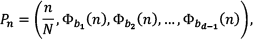
As the number of nodes in the graph increases, the PRM planner is more likely to solve queries and the failure rate decreases. On the other hand, increasing the number of samples in the roadmap degrades the efficiency of the algorithm through the growth of the planner's running time. Figure 4 illustrates the changes in the failure rate and runtime of the RPM planner in the environment shown in Figure 3 for different numbers of nodes in the PRM graph.

Figure 4.

Changes in the failure rate and runtime of the PRM planner in a bug trap workspace for different numbers of nodes.

3. A low-dispersion PRM planner

The main motivation of the low dispersion-PRM (LD-PRM) planner is to improve the dispersion of the generated samples by the original PRM algorithm so that the planner can capture the connectivity of the workspace and solve planning queries with fewer samples, which reduces the running time of the algorithm. The proposed algorithm works similarly to the original PRM with one major difference in the learning phase. In the proposed planner, the learning phase is different such that the generated samples need to fulfil an important criterion in order to be included inside the roadmap. This criterion implies that the samples are forbidden to be close to each other more than a predefined radius. Note that in this research the Euclidean distance is used. Based on the Lebesgue measure (volume) of the collision-free configuration space, we can formulize this radius as follows:

R = \frac{1}{N} \sqrt{L (Q_{f r e e}) (N - λ) / π}

[7]

where Q_free is the free configuration space, N is the number of samples (nodes) in the roadmap, and λ is a positive scaling scalar. The idea behind this formulation is that if we want to fit N non-overlapping balls inside the configuration space, the aggregate volume of these balls should be smaller than the volume of the free space. On the other hand, even if these balls are uniformly distributed in an ideal grid structure, there remain some uncovered areas in the free space because the circular shape of the balls does not cover the whole space, as illustrated in Figure 5.

Figure 5.

Ideal arrangement of the generated samples in a grid structure. Based on the shape of the samples, the environment is not covered completely.

The volume of the uncovered area in each cell of the grid is equal to R²(4 – π), which makes the total uncovered volume equal to or larger than NR²(4 – π). For N ≥ 5, and this volume is greater than the size of one cell of the grid which, in an ideal grid structure with sufficient N, is L(Q_free)/N. Recalling the fact that the total covered volume is smaller than L(Q_free), one may determine this volume as follows:

N π R^{2} \leq L (Q_{f r e e})

[8]

Therefore:

N π R^{2} = L (Q_{f r e e}) - λ \frac{L (Q_{f r e e})}{N}

[9]

which indicates that at least λ cells will remain uncovered. Hence, the value of R can be formulized as in equation 7. λ is a positive scaling integer. For the formulation to remain true, the value of λ should satisfy the following condition:

λ < N

[10]

This guarantees that at least one of the grid cells is covered after generating N samples. During the experimental studies, we found λ = N^0.5 to be the most promising value. Choosing the suitable value for λ is very important and can affect the convergence of the planner, as explained in section 5.

Now that we have a desirable value for R, we can proceed with the proposed algorithm. Algorithm 3 shows the procedure of the proposed LD-PRM planner.

As can be seen in Algorithm 3, the major difference between the original PRM and the proposed planner is in line 6, where the proposed planner checks the dispersion criterion before selecting the samples. Surprisingly, this simple adjustment improves the performance of the planner effectively in terms of the size of the graph and the runtime of the planner. The dispersion criterion prevents clumping or gaps inside the workspace by arranging the samples in a uniform and equally distributed fashion. Since the number of nodes in the resultant graph is low, the number of collision-checks and connections is reduced and the planner solves any motion planning query faster than the original PRM.

Figure 6 shows the sampling procedure of the LD-PRM planner. After selecting a sample, a ball centres at the node's position and marks that region as forbidden. Forbidden regions are illustrated with yellow circles in Figure 6.

Figure 6.

Procedure of sampling in LD-PRM. The yellow circles around each sample illustrate the forbidden regions.

The forbidden regions around each sample are illustrated by yellow circles to give a better understanding about the learning behaviour of the LD-PRM. The solution shown in Figure 6 was obtained with 30 nodes in the graph, while the simulation results show that the original PRM is not able to solve this particular case with less than 100 samples. Note that, in Figure 6, only a small section of the graph was illustrated to improve the visibility of the forbidden areas.

Algorithm 3.

LD-PRM learning phase

Generally, the main structural difference between the proposed and original PRM planners is how sparsely and uniformly the samples are distributed inside the workspace. As stated before, the PRM planner is not able to guarantee low dispersion for the resultant nodes.

Figure 7 shows the resultant samples of the PRM planner and the proposed algorithm in a 2D convex indoor environment, both with 200 nodes (N = 200). Observing Figure 7, the resultant graph of the LD-PRM algorithm is almost equally and uniformly distributed. In the next section, we discuss the advantages of the proposed planner based on the simulation results and also compare it with the original PRM and three low-dispersion variants of PRM for different types of problems.

Figure 7.

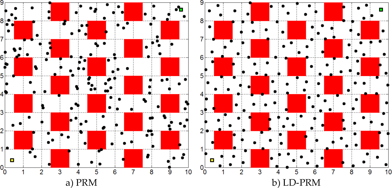
The learning phase of the original PRM and the proposed algorithm with 200 nodes.

4. Simulation studies

For testing the performance of the proposed planner and comparing it with the original PRM algorithm, we designed six different test problems. The MATLAB programming environment was used for simulation on a computer with a 3.16GHz Intel Core 2 Duo Processor. The test problems include a simple 2D environment with 22 identical convex obstacles (dim(C)=2), a 2D configuration space with a bug trap where the initial position is inside the trap (dim(C)=2), an articulated robot with three links and a moving base in an environment with six convex obstacles (dim(C)=5), and finally three variations of the d-dimensional bent corridor problem [11] with two narrow passages through which a point robot should pass to reach the goal configuration (we show the results for dim(C) =2, 3, 6)). Figure 8 presents these test problems.

Figure 8.

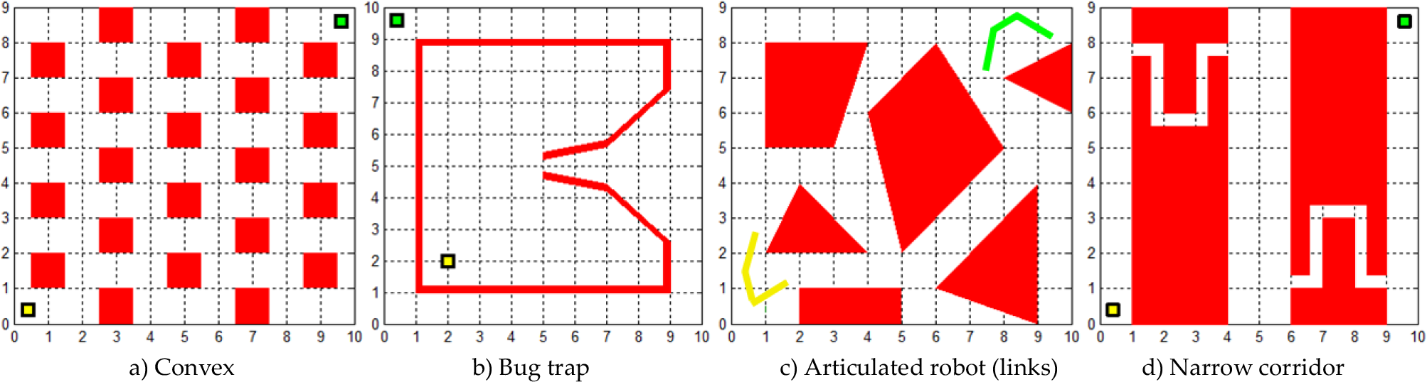
Test problems. Initial and goal configurations are illustrated with yellow and green colours, respectively.

Besides the original PRM algorithm, we used three low-dispersion variants of PRM in the simulations and comparison studies. The first algorithm employs the Hammersley sequence as the source of sampling. This method is introduced in the context of quasi-randomized path planning [12]. The second algorithm uses the Halton sequence for generating samples.

A complete study on this method is available in the literature [20]. The last algorithm is the incremental low-discrepancy lattice (ILDL) algorithm [10]. The PRM, Hammersley, Halton and ILDL algorithms were used along with the proposed LD-PRM planner to solve the planning queries of Figure 8. Table 1 presents the simulation results in terms of the number of nodes required to solve the queries and runtime of the planner.

Table 1.

Simulation results in test environments in terms of the number of nodes and runtime for the original PRM, the proposed LD-PRM and other studied algorithms. The average results have been obtained from 1,000 iterations.

	PRM (k=10)		Hammersley (k=10)		Halton (k=10)		ILDL (k=10)		LD-PRM (k=10)
	Nodes	T (sec)	Nodes	T (sec)	Nodes	T (sec)	Nodes	T (sec)	Nodes	T (sec)	R	λ
Convex (d=2)	318	5.28	133	1.13	176	1.09	176	0.89	117	0.44	0.40	10.82
Bug Trap (d=2)	1440	167.13	677	29.33	690	27.13	707	25.25	601	22.97	0.22	24.52
Links (d=5)	2312	377.14	915	45.34	1032	48.44	1004	51.16	879	36.19	0.14	29.65
Narrow (d=2)	1232	156.76	412	12.22	618	12.13	488	13.12	403	9.55	0.18	20.07
Narrow (d=3)	1834	314.65	663	56.08	792	63.02	719	60.77	608	49.34	0.15	24.66
Narrow (d=6)	4302	577.09	1549	125.33	2076	167.34	1616	154.34	1559	123.58	0.09	39.48

Based on the randomized nature of the sampling-based algorithms, the generated results in different executions of the planner are different. Therefore, we repeat each experiment 1,000 times in order to obtain the average outputs of the planners. By performing a large number of experiments, we believe that we present a more realistic characterization of the performance of the proposed LD-PRM planner. The algorithm solves planning queries in shorter runtimes by constructing smaller graphs. Among the other studied low-dispersion planners, the Hammersley sequence provides superior results in terms of runtime and graph size, while the LD-PRM outperforms the Hammersley sequence. In total, in 2D problems, the proposed planner provides solutions with effective smaller graphs.

In higher-dimensional problems, i.e., articulated robot (d=5), and narrow corridor (d=3,6), the proposed algorithm - surprisingly - provides superior results. As described before, the main aim of using deterministic sampling source is to reduce the discrepancy or dispersion of the samples. However, it has been proven that the computational cost of achieving a fixed discrepancy or dispersion grows exponentially with the dimension of the configuration space [20]. Assume a normalized configuration space C: [0,1]^d(c). In such a case, there will be N^1/d(c) intervals per axis with N samples. Considering the fact that in a typical PRM planning problem the size of the graph is usually small, it is clear that in high-dimensional problems (d(c) ≥ 3), the dispersion and discrepancy are high even if a deterministic source is used. Hence, the comparative advantage of deterministic sampling sources fades away when the dimensionality increases. With this notation about the dimensionality and sampling source, we can explain the superiority of the LD-PRM algorithm. While the Hammersley, Halton and ILDL planners focus on providing optimum discrepancy and/or dispersion through their deterministic sampling procedures, the LD-PRM algorithm insists on keeping the randomized behaviour of the original PRM and employs a heuristic criterion to achieve better uniformity and dispersion.

Figure 9 presents the comparison graphs of the proposed planner and other studied algorithms in terms of the failure rate in 2D test problems.

Figure 9.

Comparison graphs of the PRM and LD-PRM planners in terms of their failure rates in test environments.

As can be seen in Figure 9, the proposed algorithm successfully improves the performance of the original PRM. This improvement indicates that for a given number of samples, the probability of failure is reduced using the LD-PRM planner. Besides the original PRM, the proposed algorithm performs slightly better than other low-dispersion algorithms in terms of its failure rate. Furthermore, the performances were compared for fixed values of N. The proposed algorithm is based on a fixed and predetermined number of nodes and, therefore, it was compared to other studied planners with fixed sized graphs, i.e., N=100, 500 and 1,000. The simulation results are shown in Table 2.

Table 2.

Simulation results in the test environments in terms of dispersion (δ) and the failure rate for constant sizes of roadmap.

Problem	N	PRM		Ham		Hal		ILDL		LD_PRM
Problem	N	Dispersion	Failure	Dispersion	Failure	Dispersion	Failure	Dispersion	Failure	Dispersion	Failure
Convex 1	100	5.18	52%	3.32	21%	2.96	26%	2.74	19%	2.19	12%
	500	3.11	0%	1.45	0%	1.34	0%	1.36	0%	1.17	0%
	1000	0.47	0%	0.18	0%	0.16	0%	0.16	0%	0.13	0%
Bug Trap	100	5.13	100%	3.87	100%	3.65	100%	3.73	100%	3.28	100%
	500	3.02	73%	1.68	19%	1.59	13%	1.37	10%	1.21	11%
	1000	0.59	7%	0.29	0%	0.22	0%	0.27	0%	0.18	0%
Convex 2	100	4.18	100%	2.17	100%	1.88	100%	1.74	100%	1.39	100%
	500	2.59	74%	1.13	2%	1.21	1%	1.22	1%	0.95	0%
	1000	1.11	4%	0.67	0%	0.54	0%	0.59	0%	0.44	0%
Narrow Passage	100	6.24	82%	4.08	66%	3.85	89%	3.77	67%	3.29	43%
	500	4.07	44%	1.94	23%	1.65	3%	1.57	14%	1.20	0%
	1000	1.08	5%	0.43	0%	0.33	0%	0.38	0%	0.28	0%

According to Table 2, the proposed algorithm provides graphs with lower discrepancies and failure rates. Although the LD-PRM is not incremental and the size of the graph needs to be determined beforehand, the simulation results indicate that for a fixed number of nodes in the graph, it outperforms other studied planners.

5. Completeness of the proposed LD-PRM planner

In sampling-based motion planning algorithms, an interesting form of completeness is usually used for analysing the performance of a planner, namely probabilistic completeness. In this class of completeness, the planner is required to eventually find a solution if one exists.

For providing some evidence of the probabilistic completeness of the LD-PRM algorithm, we will prove that as the number of generated samples (N) increases, the uncovered volume of the configuration space will tend towards zero. In other words, with a sufficient number of samples, the LD-PRM planner almost covers the whole configuration space.

As mentioned before in section 3, the total covered volume can be calculated as follows:

N π R^{2} = L (Q_{f r e e}) - λ \frac{L (Q_{f r e e})}{N}

[11]

Hence, the total uncovered volume after generating N samples is equal to λ L(Q_free)/N. For large numbers of N, the convergence of this value strongly depends on the value of λ, as the volume of the free configuration space is constant. On the other hand, according to equation 10, the only restriction on the value of λ is to be smaller than N. Therefore, the value of λ L(Q_free)/N tends to zero as N increases, and we can conclude that with a sufficient number of samples the LD-PRM algorithm covers the entire free configuration space and, hence, that if a solution exists, it will eventually find it.

6. Conclusion and discussion

Sampling-based motion planning algorithms were considered in this research. We proposed a new learning strategy for the PRM planner. The main objective of this new learning strategy was to improve the uniformity of the generated samples to enable the planner to solve motion planning queries while generating fewer samples. Reducing the size of the roadmap will effectively decrease the running time of the algorithm. The proposed learning strategy considers the area around each selected sample as a forbidden sampling region. A virtual ball is centred at each selected sample with a radius R, which is obtained from the Lebesgue measure of the collision-free workspace, a desired cardinality of the PRM graph and a pre-defined scaling scalar. Applying this criterion on the sampling results in sparser and more distributed samples, which capture the connectivity of the workspace more efficiently.

Simulation studies showed the advantages of the proposed planner compared to the original PRM algorithm in terms of the failure rate, runtime and dispersion. Specifically, in difficult problems like narrow passages and bug traps, where the classic sampling-based methods face extensive difficulties in solving a planning query, the LD-PRM algorithm solves the motion planning problems effectively.

Furthermore, in measuring the uniformity of the resultant samples from the original PRM and the proposed LD-PRM, we designed an algorithm for measuring the dispersion value of a set of samples. The simulation results indicate that the proposed planner constructs graphs with almost a 50% improvement in terms of dispersion as compared to the original PRM planner.

References

Tsianos

K. I.

Sucan

I. A.

Kavraki

L. E.

, “Sampling-based robot motion planning: Towards realistic applications,” Computer Science Review, vol. 1, no. 1, pp. 2–11, 2007.

Karaman

Frazzoli

, “Sampling-based algorithms for optimal motion planning,” Int. Jour. of Robotics Research, vol. 30, no. 7, pp. 846–494, 2011.

Kavraki

L. E.

Svestka

Latombe

J. C.

Overmars

M. H.

, “Probabilistic roadmaps for path planning in high-dimensional configuration spaces,” IEEE Trans. on Robotics and Automation, vol. 12, no. 4, pp. 566–580, 1996.

LaValle

S. M.

Kuffner

J. J.

, “Randomized kinodynamic planning,” Int. Jour. of Robotics Research, vol. 20, no. 5, pp. 378–400, 2001.

Hsu

Jiang

Reif

Sun

, “The bridge test for sampling narrow passages with probabilistic roadmap planners,” Proc. of IEEE Int. Conf. on Robotics and Automation, pp. 4420–4426, 2003.

Boor

Overmars

M. H.

van der Stappen

A. F.

, “The Gaussian sampling strategy for probabilistic roadmap planners,” Proc. of IEEE Int. Conf. on Robotics and Automation, pp. 1018–1023, 1999.

Kurniavati

Hsu

, “Workspace importance sampling for probabilistic roadmap planning,” Proc. of IEEE Int. Conf. on Intelligent Robots and Systems, pp. 1618–1623, 2004.

Hsu

Sanchez-Ante

Sun

, “Hybrid PRM sampling with a cost-sensitive adaptive strategy,” Proc. of IEEE Int. Conf. on Robotics and Automation, pp. 3874–3880, 2005.

Thomas

Morales

Tang

Amato

N. M.

, “Biasing samplers to improve motion planning performance,” Proc. of IEEE Int. Conf. on Robotics and Automation, pp. 1625–1630, 2007.

10.

Lindemann

S. R.

LaValle

S. M.

, “Incremental low-discrepancy lattice methods for motion planning,” Proc. IEEE Int. Conf. on Robotics and Automation, pp. 2920–2927, 2003.

11.

LaValle

S. M.

Branicky

M. S.

Lindemann

S. R.

, “On the relationship between classical grid and probabilistic roadmaps,” Int. Jour. of Robotics Research, vol. 23, no. 7–8, pp. 673–692, 2004.

12.

Branicky

M. S.

LaValle

S. M.

Olson

Yang

, “Quasi-randomized path planning,” Proc. of IEEE Int. Conf. on Robotics and Automation, pp. 1481–1487, 2001.

13.

Yershova

Jaillet

Simeon

LaValle

S. M.

, “Dynamic domain RRTs: Efficient exploration by controlling the sampling domain,” Proc. of IEEE Int. Conf. on Robotics and Automation, pp. 3856–3861, 2005.

14.

LaValle

S. M.

, “Planning Algorithms,” Cambridge University Press, New York, USA, 2006.

15.

Amato

, “A randomized roadmap method for path and manipulation planning,” Proc. of IEEE Int. Conf. on Robotics and Automation, pp. 113–120, 1996.

16.

Barraquand

Kavraki

L. E.

Latombe

J. C.

T. Y.

Motwani

Raghavan

, “A random sampling scheme for path planning,” Int. Jour. of Robotics Research, vol. 16, no. 5, pp. 759–774, 1997.

17.

Kavraki

L. E.

Latombe

J. C.

, “Randomized preprocessing of configuration space for fast path planning,” Proc. IEEE Int. Conf. on Robotics and Automation, pp. 2138–2145, 1994.

18.

Cortes

Simeon

Laumond

J. P.

, “A random loop generator for planning the motions of closed kinematic chains using PRM methods,” Proc. IEEE Int. Conf. on Robotics and Automation, pp. 2141–2146, 2002.

19.

Lamiraux

Kavraki

L. E.

, “Planning paths for elastic objects under manipulation constraints,” Int. Jour. of Robotics Research, vol. 20, no. 3, pp. 188–208, 2001.

20.

Hsu

Latombe

J. C.

Kurniawati

, “On the probabilistic foundations of probabilistic roadmap planning,” Int. Jour. of Robotics Research, vol. 250, no. 7, pp. 627–643, 2006.

A Low Dispersion Probabilistic Roadmaps (LD-PRM) Algorithm for Fast and Efficient Sampling-Based Motion Planning

Abstract

Keywords

1. Introduction

2. The probabilistic roadmaps algorithm

3. A low-dispersion PRM planner

4. Simulation studies

5. Completeness of the proposed LD-PRM planner

6. Conclusion and discussion

References