Sage Journals: Discover world-class research

Abstract

Credit rating agencies and corporate lifecycles have been a subject of interest for practitioners and academics during the recent period of worldwide economic and debt crises. In this article, we examine what corporate lifespan the credit rating agencies predict. We employ the reliability theory commonly used in engineering and solve a Markov model based on the credit rating transition matrices issued by the Standard & Poor's rating agency. The results show that every company will eventually default in the long-term. However, the mean time to default differs according to the initial conditions of the model, which are represented by the initial credit rating. We considered a company as having initial speculative grades of B and CCC/C and calculated the mean time to default and the time after which the business can be considered safe, with a probability of only 50%. We also determined the probabilities of the individual rating grades. We suggest assessing corporate business cycles in probabilistic terms, taking into account all possible states and initial conditions.

Keywords

Corporate Lifecycle Stochastic Lifecycle Model Markov Models Corporate Rating Credit Rating

1. Introduction

During the recent period of economic and debt crises among the bulk of developed states, the business growth and evolution of corporate performance has received considerable academic attention. Meanwhile, credit rating agencies are becoming a subject of interest for practitioners and academics, since they are considered to be able to influence markets. While some economists claim that the judgments of rating agencies are “overrated” (for instance, [1]) or that they simply follow the market rather than anticipating events, these agencies are often perceived as powerful institutions that can influence the prices of bonds and equities of corporations (for example, [2]). Rating agencies issue credit rating grades on public or private debtors and issuers. If sufficiently accurate, the grades and transitions between them could predict corporate lifespans, providing that the credit rating sufficiently reflects corporate performance. The main question is: what corporate lifespan do the credit rating agencies predict? In this article, we try to answer this question by analysing the transition matrices published by Standard & Poor's rating agency using the Markov models commonly used in reliability analysis in engineering.

2. Theoretical framework

In this section, we will deal with the related theoretical framework: corporate credit rating, traditional approaches to modelling corporate development, reliability modelling and Markov models.

2.1 Corporate Credit Rating

A rating is an independent evaluation of subjects that produces a grade and thus allows for mutual comparison and ranking. Most often, we speak of the credit rating of a private or public debtor or issuer that has been issued by an independent credit rating agency. Among the most influential credit rating agencies, we can cite Standard & Poor's, Moody's and Fitch Group (the ‘Big Three’ credit rating agencies).

Corporate credit rating (the rating of corporate financial instruments) is an important financial indicator for potential investors. A general opinion is that a rating has the significant potential to influence market opinions on a subject. Decreasing the grade of a corporation can trigger self-fulfilling expectations [3]. Rating agencies are often criticized and sometimes accused of triggering the recent economic crisis. Another possible issue is the failure of ratings, which can take various forms [4]: the failure to predict defaults, the failure of ratings to be stable, the failure to issue a rating within the correct category of ratings, or the failure of two or more agencies to issue similar levels of rating for the same subject at the same time.

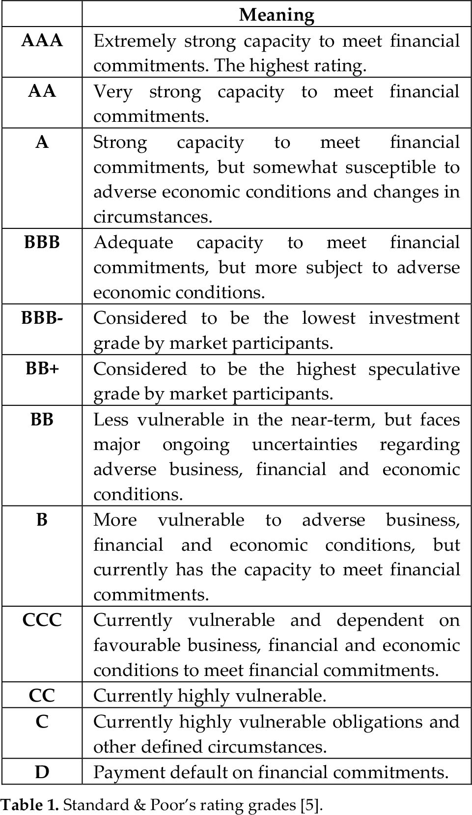
In this article, we deal with Standard & Poor's (S&P) rating grades. Nowadays, S&P issues credit ratings, which are described in detail in Table 1. Some of them may be modified by the addition of a plus (+) or minus (−) sign to show relative standings within the major rating categories.

Table 1.

Standard & Poor's rating grades [5].

	Meaning
AAA	Extremely strong capacity to meet financial commitments. The highest rating.
AA	Very strong capacity to meet financial commitments.
A	Strong capacity to meet financial commitments, but somewhat susceptible to adverse economic conditions and changes in circumstances.
BBB	Adequate capacity to meet financial commitments, but more subject to adverse economic conditions.
BBB-	Considered to be the lowest investment grade by market participants.
BB+	Considered to be the highest speculative grade by market participants.
BB	Less vulnerable in the near-term, but faces major ongoing uncertainties regarding adverse business, financial and economic conditions.
B	More vulnerable to adverse business, financial and economic conditions, but currently has the capacity to meet financial commitments.
CCC	Currently vulnerable and dependent on favourable business, financial and economic conditions to meet financial commitments.
CC	Currently highly vulnerable.
C	Currently highly vulnerable obligations and other defined circumstances.
D	Payment default on financial commitments.

In this paper, we will suppose that a corporate rating sufficiently predicts the performance of a business, thus reflecting its lifespan.

2.2 Traditional Approaches to Modelling Corporate Development

Some theorists have attempted to model the evolution of businesses using corporate lifecycles. The stage model (or corporate lifecycle theory) originated from the economic literature ([6] or [7]). This model describes the progression of a firm through multiple phases over time. For instance, we can cite five common stages of firm development [8]: birth, growth, maturity, revival and decline. However, the number of stages in corporate lifecycle models is not standardized [9]. The important thing to point out is that, from the perspective of corporate lifecycle theories, growth represents only one of the stages in the business lifecycle. Much attention has been devoted to this stage, since permanent growth is desirable and important for all for-profit organizations. Sometimes, economic theorists distinguish between two modes of growth: organic growth and growth through mergers and acquisitions (inorganic growth). In the case of small- and medium-sized firms, almost all growth is of an organic nature [10], whereas the growth of large corporations can be considered to be governed by inorganic growth.

However, empirical evidence shows that most firms do not manage to grow; instead, they enter and exit the market small (see, e.g., [11] and [12]). It is consistent with an intuitive idea, supported by the Schumpeter's theory of creative destruction [13], that it is not possible for all firms to grow; instead, only the most successful firms will manage to grow. The remaining firms are supposed to fail and eventually go out of the market. In this article, a failure of a business will be represented by its default, i.e., a failure to satisfy the terms of a loan obligation or a failure to pay back a loan (following, e.g., [14]). In many cases, the performance and lifecycle of a firm is determined by random events, thus implying the stochastic nature of corporate life. To examine the corporate lifecycle in probabilistic terms, we will employ the reliability modelling commonly used in engineering applications.

2.3 Reliability Modelling

It is not possible to assess and compare the reliability of systems without having defined the appropriate measures, because reliability itself cannot be quantified. There are multiple definitions of reliability, most of them from the field of electrical engineering. According to EPSMA [15], reliability can be defined as “the probability that a piece of equipment operating under specified conditions shall perform satisfactorily for a given period of time.” IEEE [16] defines the reliability as “the ability of a system or component to perform its required functions under stated conditions for a specified period of time.” It is important to realize that reliability is a complex property of a system, which may include susceptibility to faults, durability and maintainability, and so on, either individually or in combination with other systems. ‘Required functions’ can be defined by the set of specifications and features prescribed for the desired functionality of a system. Reliability can be expressed using reliability indicators, which have the character of random variables. Some economists have used reliability theory in the field of economics, for instance, in measuring the performance of supply chains ([17] or [18]).

A state of an object (in our model, a firm) can be either faulty (default) or fault-free (solvent). Furthermore, we can distinguish between repaired and non-repaired objects. Sometimes, when an object is in the faulty state, the failure can be repaired. Recovery/repair is the transition from the faulty to the fault-free state of an object. In this article, we will consider non-repaired systems, which means that when a firm goes into default, it cannot be recovered.

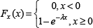
A random variable X is characterized by its distribution function F_x(x), which is the probability that the value of the random variable will be found at a value less than or equal to some given value x. Mathematically, it can be expressed as F_x(x) = P(X ≤ x). The distribution function is monotonic non-decreasing, right-continuous and takes values from 〈0,1〉. In reliability analysis, we often deal with the exponential distribution of failures, whose distribution function takes the form:

F_{x} (x) = {\begin{array}{c} 0, x < 0 \\ 1 - e^{- λ x}, x \geq 0 \end{array}

(1)

A frequently examined random variable in reliability theory is the time interval from the start-up until the failure of an object. Let t denote the time from the start-up; then, the distribution function represents the probability of the failure of the object until time t, denoted by Q(t). The complement of Q(t) represents the probability of a fault-free state until time t and is denoted by R(t). Therefore, the reliability can be expressed as:

R (t) = 1 - Q (t) .

(2)

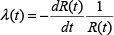
One of the most important reliability indicators is the failure rate (or, more precisely, the hazard rate in the continuous domain). It can be defined as the total number of failures within an item population, divided by the total time expended by that population during a particular measurement interval under stated conditions [19]. Using the previous definitions, the failure (hazard) rate can be specified as:

λ (t) = - \frac{d R (t)}{d t} \frac{1}{R (t)}

(3)

It follows that:

R (t) = exp (- \int_{0}^{t} λ (t) d t)

(4)

The failure rate function is commonly described using a graphical representation called the bathtub curve. This curve consists of three parts: in the first part, it is decreasing (early failures); in the second part, it is approximately constant (random failures); and in the third part, it is increasing (wear-out failures). In this article, we will consider λ(t) to be constant. In this case, R(t) is a random variable with an exponential distribution and lim_t→0 R(t) = 0. The exponential distribution is characterized by the familiar ‘memoryless’ property. In relation to the probability of failure, ‘memoryless’ means that at any given time, the probability of failure does not depend on information from the past.

Another important measure of reliability is the mean time to failure (MTTF), which we use as a measure of the mean time to default. It can be specified as:

M T T F = \int_{0}^{\infty} R (t) d t

(5)

This equation holds under the above-mentioned conditions: the exponential distribution of the random variable and constant λ(t) = λ.

2.4 Markov Models

The purpose of reliability modelling is to determine the values of the overall reliability indicators of a system based on the knowledge of the reliability indicators of its elements and their connections. Often, reliability models are divided to two classes: combinatorial models and Markov models. Markov models are based on the theory of Markov processes.

Let {X(t): t ≥ 0} be a random process with continuous time t and a discrete set of states I = {0,1,2,…,n}. The random process is a Markov process if the following property holds:

\begin{array}{l} P (X (τ) = j | X (t) = i | X (t_{n}) = i_{n}, \dots, X (t_{1}) = i_{1}) = \\ = P (X (τ) = j | X (t) = i) \end{array}

(6)

for each 0 ≤ t₁ ≤ t₂ ≤ … ≤ t_n < t ≤ τ. This property is called ‘the Markov property’. If t denotes the present time, then the probabilistic behaviour of the Markov process at an arbitrary future time τ ≥ t depends only on the present state and not on any past states. The discrete-time stochastic process with the Markov property is called ‘the Markov chain’. However, since the change in rating can be announced at any time, we consider the time to be continuous.

With homogeneous Markov processes, the probabilities of a transition between states depend only on the distance between appropriate time moments Δt = t₁ – t₂, where 〈t₁, t₂〉 denotes the interval in which the transition between two states occur.

In what follows, let p_ij(Δt) denote the probability of a transition from state i to state j over a discrete time interval Δt. A state is absorbing if, and only if, p_ii = 1 and p_ij = 0 for all i ≠ j.

Further, let λ_ij denote the intensity of a transition from state i to state j. This variable is defined as:

λ_{i j} = lim_{Δ t \to 0} \frac{p_{i j} (Δ t)}{Δ t}

(7)

and for homogeneous Markov processes, it is constant. Furthermore, for a small enough Δt, we can consider p_ij(Δt) = λ_ij(t).

For each state of a homogeneous Markov process, it is possible to construct an ordinary linear differential equation of the first-order with constant coefficients and which specifies the time function of the probability of the given state. We can formulate this equation for state i as [20]:

p_{i}^{'} (t) = \sum_{k = 0}^{\infty} p_{k} (t) λ_{k i}

(8)

where t > 0, i = 0,1,…,n and where the apostrophe denotes the first-order differentiation. A set of such equations for all states of the Markov process is called ‘the system of (forward) Kolmogorov differential equations’. It is possible to rewrite this system of equations using matrix algebra as:

p^{'} (t) = p (t) \cdot Λ

(9)

where p(t) denotes the row vector of the state probabilities and p'(t) denotes the row vector of the state probabilities of the first-order derivatives. The square matrix Λ is of order n (the number of states of the process) and is called ‘the matrix of transition rate’ (transition matrix). The element λ_ij of this matrix represents the rate of transition from state i to state j, i ≠ j. The sum of row elements is equal to zero for all rows, which means that λ_ii equals the negative value of the sum of all other row elements. For an absorbing state, the appropriate row contains only zero elements.

The initial conditions of equation (8) correspond to the initial probabilities of the individual states. Equation (9) will be used in the analysis of those Markov models that contain the absorbing states.

Repaired systems do not generally include absorbing states. In this case, it is possible to determine the steady values p_i(∞). Following [21], equation (8) takes the form of a linear system of equations for t → 0 and, in matrix algebra, can be rewritten as:

0 = p \cdot Λ

(10)

where p = p(∞) = (p₁,p₂,…,p_n) is the vector of the steady probabilities of individual states and 0 is the null vector. This homogeneous system of linear equations is linearly dependent and it can be solved after adding the normalization condition:

\sum_{j = 1}^{n} p_{i j} = 1

(11)

Markov models are based on the decomposition of a system into a set of states, among which transitions occur. The whole system can be described using the state diagram, which is a regular, directed, connected, weighted and oriented graph. The nodes of the graph represent the states of a system; the edges are weighted according to the transition rates. A state is called ‘absorbing’ if there does not exist an edge from this state to another. A simple Markov model of a non-repaired system can be illustrated using Fig. 1.

Figure 1.

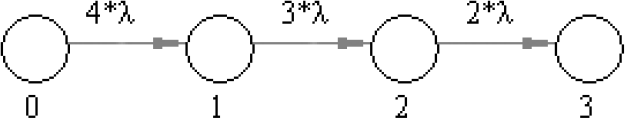
A simple Markov model.

This model simulates a system that consists of four elements, out of which only two may be broken. The model has four states, 0, 1, 2 and F, and appropriate transition rates (failure rates) denoted by λ. In the states 0, 1, 2, the system is operational, whereas in the absorbing state F, the system is broken. The matrix of the transition rates is:

Λ = (\begin{array}{l} - 4 λ & 4 λ & 0 & 0 \\ 0 & - 3 λ & 3 λ & 0 \\ 0 & 0 & - 2 λ & 2 λ \\ 0 & 0 & 0 & 0 \end{array}) .

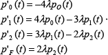
For this matrix, we can construct the system of ordinary differential equation as follows:

\begin{array}{l} p_{0}^{'} (t) = - 4 λ p_{o} (t) \\ p_{0}^{'} (t) = 4 λ p_{o} (t) - 3 λ p_{1} (t) . \\ p_{2}^{'} (t) = 3 λ p_{1} (t) - 2 λ p_{2} (t) \\ p_{F}^{'} (t) = 2 λ p_{2} (t) \end{array}

3. Methodology and results

3.1 Basic Assumptions

The model is based on the idea that a firm's default probability is driven by shocks of a regional, sectorial and industrial nature, whose arrivals can be modelled by independent homogeneous Poisson processes. Let T₁,T₂,…,T_n denote the arrival times of an event. We call this sequence a homogeneous Poisson process with intensity λ, if the differences T_t+1 – T_n are independent and exponentially distributed with parameter λ.

In the model, a default is considered to be governed by a Poisson process, which implies that the default time is subject to exponential distribution with default intensity λ (following, for instance, [22]). A Poisson process is a case of a Markov process. An efficient estimator of the intensity λ is [20]:

\hat{λ} = \frac{n}{T} \approx p

(12)

where T denotes the number of observations, n denotes the number of observed values during the period and p denotes the probability of such observed values.

Now let us summarize the assumptions considered so far:

The corporate rating sufficiently reflects the performance of a business and its lifespan [14];

If a firm goes into default, it cannot be recovered (this assumption is consistent with the definition of S&P's D state);

The default times are exponentially distributed with parameter λ [22];

The transitions between grades can be represented by a stochastic process with the Markov property ([23] or [24]);

The failure rate λ(t) = λ is constant over time, and thus the Markov process is homogeneous (we take the average value over 30 years, as described below).

3.2 Data Description

The data were taken from a global average corporate one-year transition probability matrix published by S&P in 2011. The matrix contains eight grades (AAA, AA, A, BBB, BB, B, CCC/C, D) with average one-year transition probabilities for the period 1981-2010. The probabilities are listed in Table 2.

Table 1.

Global average corporate one-year transition probabilities [5].

	AAA	AA	A	BBB	BB	B	CCC/C	D
AAA	87.9%	8.08%	0.54%	0.05%	0.08%	0.03%	0.05%	0.00%
AA	0.57%	86.4%	8.19%	0.53%	0.06%	0.08%	0.02%	0.02%
A	0.04%	1.90%	87.3%	5.37%	0.38%	0.17%	0.02%	0.08%
BBB	0.01%	0.13%	3.71%	84.5%	3.99%	0.66%	0.15%	0.25%
BB	0.02%	0.04%	0.17%	5.22%	75.6%	7.33%	0.76%	0.95%
B	0.00%	0.04%	0.14%	0.23%	5.49%	73.1%	4.49%	4.72%
CCC/C	0.00%	0.00%	0.19%	0.28%	0.83%	13.0%	43.8%	27.4%
D	0.00%	0.00%	0.00%	0.00%	0.00%	0.00%	0.00%	0.00%

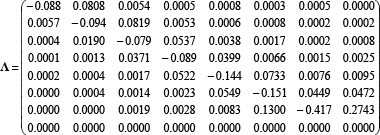
The rating grades represent discrete states in the Markov model to be analysed. The model has one absorbing state (D). Using Table 3 and assuming that λ_ij ≈ p_ij and that the row sum in the transition matrix must equal zero, we obtain the transition matrix:

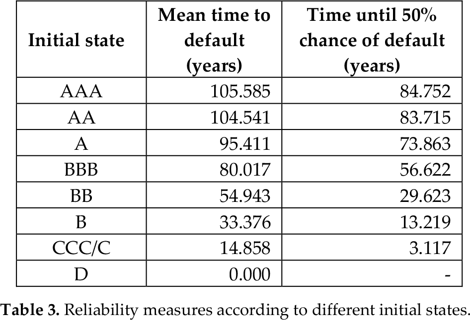
Λ = (\begin{matrix} - 0.088 & 0.0808 & 0.0054 & 0.0005 & 0.0008 & 0.0003 & 0.0005 & 0.0000 \\ 0.0057 & - 0.094 & 0.0819 & 0.0053 & 0.0006 & 0.0008 & 0.0002 & 0.0002 \\ 0.0004 & 0.0190 & - 0.079 & 0.0537 & 0.0038 & 0.0017 & 0.0002 & 0.0008 \\ 0.001 & 0.0013 & 0.0371 & - 0.089 & 0.0399 & 0.0066 & 0.0015 & 0.0025 \\ 0.0002 & 0.0004 & 0.0017 & 0.0522 & - 0.0144 & 0.0733 & 0.0076 & 0.0095 \\ 0.0000 & 0.0004 & 0.0014 & 0.0023 & 0.0549 & - 0.151 & 0.0449 & 0.0472 \\ 0.0000 & 0.0000 & 0.0019 & 0.0028 & 0.0083 & 0.1300 & - 0.417 & 0.2743 \\ 0.0000 & 0.0000 & 0.0000 & 0.0000 & 0.0000 & 0.0000 & 0.0000 & 0.0000 \end{matrix})

Table 3.

Reliability measures according to different initial states.

Initial state	Mean time to default (years)	Time until 50% chance of default (years)
AAA	105.585	84.752
AA	104.541	83.715
A	95.411	73.863
BBB	80.017	56.622
BB	54.943	29.623
B	33.376	13.219
CCC/C	14.858	3.117
D	0.000	–

Finally, the whole Markov model of the corporate lifespan is depicted in Fig. 2.

Figure 2.

A Markov model of the corporate lifespan.

3.3 Results and Discussion

We used MATLAB to numerically solve the system's Kolmogorov differential equations resulting from (8) and (9), and to calculate the MTTF, which represents the mean time to default and the probabilities of the individual rating states. We obtained a probabilistic model of the corporate development with individual states and their probabilities.

Firstly, we show that the mean time to default varies according to the initial grade, as well as the time when a company cannot be deemed to be safe anymore. The results are listed in Table 3.

Generally, it is considered that the average lifespan of a company is shorter than 50 years [25] and that it is - possibly - continuously decreasing to about 25 years [26]. This corresponds to the initial state B or CCC/C, which is an acceptable assumption, since new market entrants can indeed be considered to be in highly speculative grades. Further, we consider a “new-entrant” company to have the initial B or CCC/C speculative grades. Using these initial conditions, we obtain a MTTF of 33.376 years for the state B and of 14.858 years for the state CCC/C.

The reliability functions defined in equations (1) and (2) are shown in Fig. 3.

Figure 3.

The reliability function R(t) and the probability of default Q(t).

This figure shows that the S&P rating, in the long-term, predicts unavoidable default for these companies and that the probability of default is growing rapidly. Conversely, the reliability (i.e., the ability of a corporation to meet its long-term fixed expenses and to accomplish long-term expansion and growth) is rapidly decreasing. The shift from the initial state B to a riskier initial state CCC/C results in a considerable decrease of reliability.

The probabilities of the states AAA, AA, A, BBB, BB, B, CCC/C and D are shown in Fig. 4 for the two initial states. The vertical sum of all the curves equals one. From the upper part of the figure, it is evident than the probability of staying in the initial state is rapidly decreasing during the first few years. Meanwhile, the probability of default is rapidly increasing, and after a few years it exceeds 50% (13.219 years for the state B, 3.117 years for the state CCC/C). These curves have typical exponential shapes.

Figure 4.

Time plot of probabilities.

In the lower part of the figure, we can see that the time plots of the probabilities of some of the other states resemble the classic business cycle shape. However, these probabilities are considerably lower than the probability of default (D).

It is important to realize that we chose the initial conditions according to the speculative states B and CCC/C; the results would be much more favourable for a company starting in the AAA state, as suggested by Table 3. In particular, the probability of default for a company starting with the AAA grade is very low during the first 30 years. However, the fact that a company is ultimately condemned to default is not affected by the choice of initial states.

4. Conclusion

In this article, we tried to answer the initial question: what corporate lifecycle do the credit rating agencies predict? To answer this question, we employed the reliability theory commonly used in engineering and we solved the problem using a Markov model based on the credit rating data issued by the Standard & Poor's rating agency.

Our model shows that each surveyed company will eventually default in the long-term. However, the mean time to default differs according to the initial conditions of the model, which are represented by the initial credit rating. We determined the mean time to default for the AAA, AA, A, BBB, BB, B, CCC/C and D initial states, and the time after which they cannot be deemed safe with more than a 50% probability. Next, we considered a ‘new-entrant’ company having an initial B or CCC/C speculative grade. We found that the shift from the initial state B to the riskier initial state CCC results in a considerable decrease of reliability and that the probability of staying in the initial state rapidly decreases during the first few years. We also determined the probabilities of individual rating grades as functions of time. However, the results would be much more favourable if the initial state belonged to the higher rating categories. We suggest assessing corporate business cycles in probabilistic terms, taking into account all possible states and initial conditions.

The model has to fulfil several assumptions. We believe that corporate ratings sufficiently reflect the performance of businesses and their corporate lifespans. The assumption that if a firm goes in default, it cannot be recovered, is consistent with the definition of the Standard & Poor's D state. The more constraining assumptions are that the default times are exponentially distributed, that the transitions between grades can be represented by a stochastic process with the Markov property, and that the Markov process is homogeneous.

This article is intended to contribute to the issue of rating agencies' predictions and corporate lifecycles, which are becoming important topics of interest in light of the contemporary worldwide financial and debt crises.

Footnotes

5. Acknowledgements

This article was written with financial support from the Internal Grant Agency of the University of Economics, Prague, project no. F3/9/2013.

References

Hilscher

Wilson

(2011) Credit ratings and credit risk. Brandeis University Working Papers No. 31.

Norden

(2008) Credit Derivatives. Corporate News and Credit Ratings. University of Mannheim Working Paper, 18th October 2008.

Gärtner

Griesbach

(2012) Rating agencies, self-fulfilling prophecy and multiple equilibria? An empirical model of the European sovereign debt crisis 2009-2011. University of St. Gallen, Economics Working Paper No. 1215.

Minescu

A.M

(2010) A Study on the failure of sovereign credit ratings. The Business Review Cambridge 16(2).

Standard & Poor's (2011) Quarterly Global Corporate Default Update and Rating Transitions. Available online: http://www.standardandpoors.com/ratings/articles/en/us/?articleType=HTML&assetID=1245324135356

Penrose

E.T

(1952) Biological analogies in the theory of the firm. American Economic Review 42(5): 804–819.

Rostow

W.W

(1960) The Stages of Economic Growth. Cambridge: Cambridge University Press.

Miller

Friesen

P.H

(1984) A longitudinal study of the corporate lifecycle. Management Science 30(10): 1161–1183.

Lester

D.L

Parnell

J.A

Crandall

Menefee

M.L

(2008) Organizational lifecycle and performance among SMEs: Generic strategies for high and low performers. International Journal of Commerce and Management 18(4): 313–330.

10.

Davidsson

Delmar

(1998) Some important observations concerning job creation by firm size and age. Paper presented at the Rencontres St. Gall, September 1998, Gallen, Switzerland.

11.

Reynolds

P.D

White

S.B

(1997) The entrepreneurial process: economic growth, men, women and minorities. Westport: Quorum Books.

12.

Samuelsson

(2001) Modeling the nascent venture opportunity exploitation process across time. In Bygrave

W.D

, editors. Frontiers of Entrepreneurship Research, Wellesley: Babson College, pp. 66–79.

13.

Schumpeter

J.A

(1942) Capitalism, Socialism and Democracy. New York: Harper & Row.

14.

Zeitun

Tian

Keen

(2007) Default probability for Jordanian companies: A test of cash flow theory. International Research Journal of Finance and Economics 8: 147–162.

15.

European Power Supply Manufacturers Association (EPSMA) (2005) Reliability: Guidelines to Understanding Reliability Prediction. Available online: http://www.epsma.org/pdf/MTBF%20Report_24%20June%202005.pdf

16.

Institute of Electrical and Electronics Engineers (IEEE) (1990) IEEE Standard Computer Dictionary: a Compilation of IEEE Standard Computer Glossaries. New York: IEEE.

17.

Cao

(2008) Reliability analysis and evaluation on the member enterprises of a manufacturing supply chain based on a BP neural network. Paper presented at the 15th International Conference on Management Science and Engineering, September 2008, Long Beach, USA.

18.

Klimov

Merkuryev

(2008) Simulation model for supply chain reliability evaluation. Technological and Economic Development of Economy 14(3): 300–331.

19.

MacDiarmid

(1995) Reliability Toolkit: Commercial Practices Edition. New York and Rome: Reliability Analysis Center and Rome Laboratory.

20.

Rektorys

(1995) An Overview of Applied Mathematics 2. Prague: Prometheus.

21.

Hlavička

(1992) Fault Tolerant Digital Systems. Prague: Czech Technical University Publishing House.

22.

D.X

(2000) On default correlation: A copula function approach. Journal of Fixed Income 9(4): 43–54.

23.

Belkin

Forest

Suchower

(1998) A one-parameter representation of credit risk transition matrices. CreditMetrics Monitor Third Quarter, pp. 44–56.

24.

Kiefer

Larson

(2004) Testing simple Markov structures for credit rating transition. Comptroller of the Currency, Economic and Policy Analysis Working Paper.

25.

De Geus

(1997) The Living Company. Boston: Harvard Business School Press.

26.

Morris

(2003) Business Model Warfare: The Strategy of Business Breakthroughs. Philadelphia: Innovation Labs & ACASA.

A Stochastic Model of Corporate Lifespan Based on Corporate Credit Ratings