Sage Journals: Discover world-class research

Abstract

This paper deals with the modelling, simulation-based controller design and path planning of a four rotor helicopter known as a quadrotor. All the drags, aerodynamic, coriolis and gyroscopic effect are neglected. A Newton-Euler formulation is used to derive the mathematical model. A smart self-tuning fuzzy PID controller based on an EKF algorithm is proposed for the attitude and position control of the quadrotor. The PID gains are tuned using a self-tuning fuzzy algorithm. The self-tuning of fuzzy parameters is achieved based on an EKF algorithm. A smart selection technique and exclusive tuning of active fuzzy parameters is proposed to reduce the computational time. Dijkstra's algorithm is used for path planning in a closed and known environment filled with obstacles and/or boundaries. The Dijkstra algorithm helps avoid obstacle and find the shortest route from a given initial position to the final position.

Keywords

Quadrotor PID Fuzzy Extended Kalman Filter Self-Tuning Smart Selection

1. Introduction

A quadrotor is a cross-shaped aerial vehicle that is capable of vertical take-off and landing. It has four motors, each mounted per corner equidistant from the centre. The synchronized rotational speed (ω) of all the motors is key to the control of the quadrotor. Vertical motion results from the simultaneous increase or decrease of the rotational speeds of all the rotors. The motion along any direction on the lateral axis is obtained by decreasing the rotational speed of the rotors along the desired direction of motion, and increasing the rotational speed of the rotors opposite to the desired direction of motion. Moment produced by rotation of rotors is used to initiate yaw. For instance, clockwise yaw is initiated by simultaneously increasing the rotation speed of the rotors creating a clockwise moment, and decreasing the rotation speed of the rotors creating counterclockwise moment. The motion of the quadrotor is described schematically in figure 1. Control of a quadrotor is a challenging task for the following reasons: high manoeuvrability, high non-linearity, intensely coupled multivariable and under-actuated condition with six degrees of freedom and only four actuators.

Figure 1.

Basic motion of a quadrotor.

A quadrotor is not a new concept. The first successful hovering of a quadrotor was achieved in October 1920 by Dr. George de Bothezat and Ivan Jerome [1]. Researchers have designed and implemented numerous quadrotor controllers such as PID/PD controllers, fuzzy controllers, sliding mode controllers, neuro-fuzzy controllers and vision-based controllers. M. Santos et al. [2] proposed an intelligent system based on fuzzy logic to control a quadrotor. C. Coza et al. [3] used an adaptive fuzzy control algorithm to control a quadrotor in the presence of sinusoidal wind disturbance. The author addressed a robust method to prevent drift in the fuzzy membership centres. Y. A. Younes et al. [4] introduced a backstepping fuzzy logic controller as a new approach to controlling the attitude stabilization of a quadrotor. The backstepping controller parameters were scheduled utilizing fuzzy logic. M. H. Amoozgar et al. [5] proposed an adaptive PID controller for fault-tolerant control of a quadrotor helicopter in the presence of actuator faults. The PID gains were tuned using a fuzzy interface scheme. A. Sharma et al. presented and compared PID and fuzzy PID controllers to stabilize a quadrotor. Other authors [6 –8] also addressed the fuzzy PID control algorithm to control a quadrotor.

In this paper, modelling of a quadrotor, a control strategy using a self-tuning fuzzy PID algorithm and path planning using Dijkstra's algorithm are presented. A dynamic model is derived based on the Euler-Newton formulation. All the drags, aerodynamic, Coriolis and gyroscopic effects are neglected. The PID gain scheduling-based control algorithm is proposed for attitude stabilization and position control of the quadrotor. The tuning of PID gains is performed based on the self-tuning fuzzy controller. The tuning of the fuzzy parameters is performed using an EKF algorithm. Smart selection of the active fuzzy parameter followed by exclusive tuning of the active parameter is proposed to reduce the computational time. A path planning algorithm is proposed with two main objectives in mind: obstacle avoidance and shortest route calculation from any given initial position to the final position. Finally, a series of simulation results and conclusions are presented.

2. Mathematical Modelling

The mathematical model of the quadrotor is derived based on the Newton-Euler formulation. Let E = X_E, Y_E, Z_E denote an inertial frame and B = X_B,Y_B,Z_B denote a body fixed frame. The body frame is related to the inertial frame by a position vector (x, y, z) and three Euler angles, (φ, θ, ψ) representing roll, pitch and yaw respectively. All equations are expressed in the inertial frame. The vehicle is assumed to be rigid and symmetrical. The centre of mass, centre of gravity and origin of body axis are assumed to be coincident. Let cφ represent cos φ, and sφ represent sin φ. Similar notation is used for θ and ψ. The rotation matrix from the body frame to the inertial frame $_{B}^{E} R$ for the defined coordinate system is computed by multiplying the three matrices $_{B}^{E} R_{X}$ , $_{B}^{E} R_{Y}$ and $_{B}^{E} R_{X}$ generated by rotations about the X_B, Y_B and Z_B axes respectively.

Figure 2.

Coordinate system.

\begin{array}{l} ​_{B}^{E} R =_{B}^{E} R_{Z} \times_{B}^{E} R_{Y} \times_{B}^{E} R_{X} \\ ​_{B}^{E} R = [\begin{matrix} c ψ & - s ψ & 0 \\ s ψ & c ψ & 0 \\ 0 & 0 & 1 \end{matrix}] \times [\begin{matrix} c θ & 0 & s θ \\ 0 & 1 & 0 \\ - s θ & 0 & c θ \end{matrix}] \times [\begin{matrix} 1 & 0 & 0 \\ 0 & c φ & s φ \\ 0 & - s φ & c φ \end{matrix}] \\ ​_{B}^{E} R = [\begin{matrix} c θ c ψ & - s φ s θ c ψ - c φ s ψ & c φ s θ c ψ - s φ s ψ \\ c θ s ψ & - s φ s θ s ψ + c φ c ψ & c φ s θ s ψ + s φ c ψ \\ - s θ & - s φ c θ & c φ c θ \end{matrix}] \end{array}

(1)

The rotation of each rotor produces a vertical force towards the Z_B direction and moment is produced opposite to the direction of rotation. Rotors are paired such that the total moment created is cancelled out. The rotor pair 2-4 produces clockwise moment, while the rotor pair 1-3 creates counterclockwise moment. Experimental observation at low speed showed that these moments are linearly dependent on the produced forces. The equation of motion can be written using force and moment balance as shown in equation 2 [9 –11]

[\begin{matrix} \overset{..}{x} \\ \overset{..}{y} \\ \overset{..}{z} \\ \overset{..}{φ} \\ \overset{..}{θ} \\ \overset{..}{ψ} \end{matrix}] = (\begin{matrix} ​_{B}^{E} R {[\begin{matrix} 0 \\ 0 \\ \sum F_{i} \end{matrix}] - [\begin{matrix} K_{1} \dot{x} \\ K_{2} \dot{y} \\ K_{3} \dot{z} \end{matrix}]} \frac{1}{m} - [\begin{matrix} 0 \\ 0 \\ g \end{matrix}] \\ {\begin{matrix} l (F_{1} - F_{2} - F_{3} + F_{4} + K_{4} \dot{ϕ}) / I_{X} \\ l (- F_{1} - F_{2} + F_{3} + F_{4} + K_{5} \dot{θ}) / I_{Y} \\ (C F_{1} - C F_{2} + C F_{3} - C F_{4} + K_{6} \dot{ψ}) / I_{Z} \end{matrix} \end{matrix})

(2)

where M_i = C × F_i, F_i is the force from individual motors, M_i is the moment produced by rotation of the rotor for i = 1, …,4, C is the constant relating moment to force, m is the total mass of the UAV, g is the acceleration due to gravity, K_i is the coefficient of the drag opposing the motion of the quadrotor, for i = 1,2,…, 6. I_X, I_Y, I_Z are the moment of inertia of the UAV with respect to X_B, Y_B, Z_B axes respectively. As the drags are negligible at low speed, for convenience the drag coefficients are assumed to be zero [9]. Moreover, inputs are defined as:

U = [\begin{matrix} U_{1} \\ U_{2} \\ U_{3} \\ U_{4} \end{matrix}] = [\begin{matrix} \frac{1}{m} \sum_{i = 1}^{4} F_{i} \\ \frac{1}{I_{X}} (F_{1} - F_{2} - F_{3} + F_{4}) \\ \frac{1}{I_{Y}} (- F_{1} - F_{2} + F_{3} + F_{4}) \\ \frac{C}{I_{Z}} \sum_{i = 1}^{4} {(- 1)}^{i + 1} F_{i} \end{matrix}]

(3)

Substituting equation 3 to equation 2, the simplified form of the quadrotor dynamics is obtained as presented in equation 4.

{\begin{array}{l} \overset{..}{x} = U_{1} (c φ s θ c ψ - s φ s ψ) \\ \overset{..}{y} = U_{1} (c φ s θ s ψ + s φ c ψ) \\ \overset{..}{z} = U_{1} (c φ c θ) - g \\ \overset{..}{φ} = U_{2} l \\ \overset{..}{θ} = U_{3} l \\ \overset{..}{ψ} = U_{4} \end{array}

(4)

Likewise, the motor is modelled considering a small motor with very low inductance and no gearbox. The motor dynamics is given by equation 5 [10, 11]

J \dot{ω} = - \frac{K_{E} K_{M}}{R} ω - d ω^{2} + \frac{K_{M}}{R} V

(5)

where J is the propeller inertia, ω is the rotational speed, K_E is the back EMF constant, K_M is the torque constant, R is the internal resistance of the motor, d is the aerodynamic drag factor and V is the motor input voltage.

3. Control and Path Planning Algorithm

3.1. Self-Tuning Fuzzy PID

A PID (Proportional-Integral-Derivative) controller is a well-known feedback controller most widely used in various types of plants and industries utilizing robotics all over the world. A PID controller is simple and easy to design which often results in satisfactory performance. However, a PID controller has various limitations: the fixed gains of a PID controller limits the performance over a wider range of operating points. As a PID controller is based on the linear model, non-linearity in the system brings uncertainty and degraded performance. It lacks learning ability and the adaptability necessary to overcome nonlinearities and uncertainties. So, gain scheduling of a PID controller based on self-tuning of fuzzy parameters [12, 13] is proposed. The proposed algorithm can be described as presented in figure 3. The quadrotor is controlled using a PID algorithm. The proportional, derivative and integral gains of the PID controller are tuned using fuzzy logic. The fuzzy parameters of the fuzzy algorithm are further tuned using an EKF algorithm.

PID output is defined by,

U_{P I D} = k_{p} e (t) + k_{i} \int e (t) d t + k_{d} \dot{e} (t)

(6)

Figure 3.

Control algorithm structure.

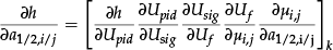
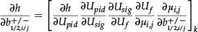
where k_p, k_i, k_d are PID gains, e (t) is error from reference to response signal at time t. The PID gains k_a are tuned across range Δk_a based on the input variables error e (t) and its first derivative ė (t) as given by equation 7

k_{a} = k_{a_0} + U_{s i g} \times Δ k_{a}

(7)

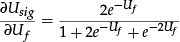
where k_{a_}₀ is the base value of the gain. U_sig ∈ [0,1] is the normalized output from the sigmoid function defined as:

U_{s i g} = \frac{1 - e^{- U_{f}}}{1 + e^{- U_{f}}}

(8)

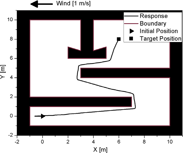
where U_f is the output from fuzzy logic. Inputs to the fuzzy logic are normalized on range [-1 1]. For each input variables, five equal-sized isosceles triangular membership functions are considered NB, NS, ZE, PS, PB representing negative big, negative small, zero, positive small and positive big respectively. The membership function for each output is considered to be five singleton values. Details of membership functions are represented in figure 4.

Figure 4.

a) Input membership functions b) Output singleton values.

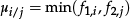
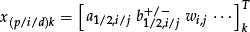
Let, i and j represent the membership function index for the first and second input variables. Three vertices are used to define each of the triangular membership functions. (a_1/2,i/j, 1) be the top vertices, (a_1/2,i/j − b⁻_1/2,i/j, 0) and (a_1/2,i/j + b⁺_1/2,i/j, 0) represent the base vertices. Each crisp input is fuzzified according to equation 9 to obtain the membership grade value f_1/2,i/j for i^th or j^th membership function.

f_{1 / 2, i / j} = {\begin{array}{l} 1 + \frac{O f f s e t_{i / j}}{b_{1 / 2, i / j}^{-}} \begin{matrix} , i f & 0 ⩾ O f f s e t_{i / j} ⩾ - b_{1 / 2, i / j}^{-} \end{matrix} \\ 1 - \frac{O f f s e t_{i / j}}{b_{1 / 2, i / j}^{+}} \begin{matrix} , i f & 0 ⩽ O f f s e t_{i / j} ⩽ b_{1 / 2, i / j}^{+} \end{matrix} \\ 0 \begin{matrix} \begin{matrix} O t h e r w i s e \end{matrix} \end{matrix} \end{array}

(9)

where Offset_i/j = x_1/2 − a_1/2,i/j is defined as the distance vector from the tip vortex of the triangular membership function to the corresponding input x₁ or x₂ being error and error rate respectively.

Based on experience, 25 fuzzy rules are defined for all possible combinations of the inputs. These defined rules are used for initial calculation and are later tuned based on the system response. A minimum function is used to define the connectives. The output membership grade is obtained by equation 10.

μ_{i / j} = \min (f_{1, i}, f_{2, j})

(10)

Defuzzification to the crisp value is done using the centre of gravity method for singletons (COGS).

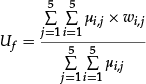
U_{f} = \frac{\sum_{j = 1}^{5} \sum_{i = 1}^{5} μ_{i, j} \times w_{i, j}}{\sum_{j = 1}^{5} \sum_{i = 1}^{5} μ_{i, j}}

(11)

where w_i,j is a weighted singleton value from rule table. The fuzzy rules and membership functions are tuned based on the EKF algorithm. The states in the EKF estimation are as presented in equation 12

x_{(p / i / d) k} = {[\begin{matrix} a_{1 / 2, i / j} & b_{1 / 2, i / j}^{+ / -} & w_{i, j} & \dots \end{matrix}]}_{k}^{T}

(12)

Equation 13 describes the system model and the measurement model.

{\begin{matrix} x_{k + 1} = f (x_{k}) + w_{k} \\ z_{k} = h (x_{k}) + v_{k} \end{matrix}

(13)

where x_k represents the fuzzy states at sampling time k, and z_k. is the measurement as obtained from the sensors. w_k and v_k are the process and measurement noise which are both assumed to be uncorrelated zero mean Gaussian noises with covariance Q_k. and R_k respectively. Function f is the state transition model used to compute the predicted state from the current state estimate h represents the measurement model with respect to the estimated states which is as presented in equation 14.

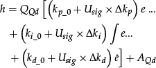
\begin{array}{l} h = Q_{Q_{d}} [(k_{p_0} + U_{s i g} \times Δ k_{p}) e \dots \\ + (k_{i_0} + U_{s i g} \times Δ k_{i}) \int e \dots \\ + (k_{d_0} + U_{s i g} \times Δ k_{d}) \dot{e}] + A_{Q_{d}} \end{array}

(14)

where Q_Qd is the quotient term to the inputs U1, U2, U3 and U4 as in the quadrotor dynamics equation 2. Similarly the term A_Qd is the additive term in the equation 2. For the extended Kalman filter, initial values of the states are supposed to be known precisely thus setting the initial error covariance (P⁻) to zero. The measurement model is linearized using the Jacobian as expressed in equation 15.

H_{k} = {\frac{\partial h}{\partial x_{i}} |}_{k} = {[\begin{matrix} \frac{\partial h}{\partial a_{1 / 2, i / j}} & \frac{\partial h}{\partial b_{​_{1 / 2, i / j}}^{+ / -}} & \frac{\partial h}{\partial w_{i, j}} \end{matrix}] |}_{k}

(15)

The term $\partial h \partial a_{1 / 2, i / j}$ in equation 15 can be calculated as

\frac{\partial h}{\partial a_{1 / 2, i / j}} = {[\frac{\partial h}{\partial U_{p i d}} \frac{\partial U_{p i d}}{\partial U_{s i g}} \frac{\partial U_{s i g}}{\partial U_{f}} \frac{\partial U_{f}}{\partial μ_{i, j}} \frac{\partial μ_{i, j}}{\partial a_{1/2,i/j}}]}_{k}

(16)

where,

{\frac{\partial h}{\partial U_{p i d}} |}_{k} = \frac{h_{k} - h_{k - 1}}{U_{p i d_{k}} - U_{p i d_{k - 1}}}

(17)

\frac{\partial U_{p i d}}{\partial U_{s i g}} = {\begin{array}{l} Δ k_{p} \times e (t) f o r p - T u n e r \\ Δ k_{i} \times \int e (t) f o r i - T u n e r \\ Δ k_{d} \times \frac{d e (t)}{d t} f o r d - T u n e r \end{array}

(18)

\frac{\partial U_{s i g}}{\partial U_{f}} = \frac{2 e^{- U_{f}}}{1 + 2 e^{- U_{f}} + e^{- 2 U_{f}}}

(19)

\frac{\partial U_{f}}{\partial μ_{i, j}} = \frac{\sum_{m = 1}^{5} \sum_{n = 1}^{5} μ_{m, n} (w_{i, j} - w_{m, n})}{{(\sum_{m = 1}^{5} \sum_{n = 1}^{5} μ_{m, n})}^{2}}

(20)

For

\frac{\partial μ_{i, j}}{\partial f_{1 / 2, i, j}} = 1

(21)

\frac{\partial μ_{i, j}}{\partial a_{1/2,i/j}} = \frac{\partial μ_{i, j}}{\partial f_{1 / 2, i, j}} \frac{\partial f_{1 / 2, i / j}}{\partial a_{1 / 2, i / j}} = \frac{s i g n [x_{1 / 2} - a_{1 / 2, i / j}]}{b_{1 / 2, i / j}^{- / +}}

(22)

Similarly, the term $\frac{\partial h}{\partial b_{_{1 / 2, i / j}}^{- / +}}$ in equation 15 is computed as

\frac{\partial h}{\partial b_{​_{1 / 2, i / j}}^{+ / -}} = {[\frac{\partial h}{\partial U_{p i d}} \frac{\partial U_{p i d}}{\partial U_{s i g}} \frac{\partial U_{s i g}}{\partial U_{f}} \frac{\partial U_{f}}{\partial μ_{i, j}} \frac{\partial μ_{i, j}}{\partial b_{​_{1 / 2, i / j}}^{+ / -}}]}_{k}

(23)

where the terms $\frac{\partial h}{\partial U_{p i d}}$ , $\frac{\partial U_{f}}{\partial μ_{i, j}}$ , are as defined in equation 17, 18, 19 and 20

\frac{\partial μ_{i, j}}{\partial b_{​_{1 / 2, i / j}}^{+ / -}} = \frac{\partial μ_{i, j}}{\partial f_{1 / 2, i, j}} \frac{\partial f_{1 / 2, i / j}}{\partial b_{1 / 2, i / j}^{- / +}} = \frac{| x_{1 / 2} - a_{1 / 2, i / j} |}{{(b_{1 / 2, i / j}^{- / +})}^{2}}

(24)

And the term $\frac{\partial h}{\partial w_{i, j}}$ in equation 15 is computed as

\frac{\partial h}{\partial w_{i, j}} = {[\frac{\partial h}{\partial U_{p i d}} \frac{\partial U_{p i d}}{\partial U_{s i g}} \frac{\partial U_{s i g}}{\partial U_{f}} \frac{\partial U_{f}}{\partial w_{i, j}}]}_{k}

(25)

where, $\frac{\partial U_{s i g}}{\partial U_{f}}$ are defined in equation 17, 18 and 19

\frac{\partial U_{f}}{\partial w_{i, j}} = \frac{μ_{i, j}}{\sum_{i = 1}^{5} \sum_{j = 1}^{5} μ_{i, j}}

(26)

The Kalman Gain is computed as:

K_{k} = P_{k}^{-} H_{k}^{T} {(H_{k} P_{k}^{-} H_{k}^{T} + R_{k})}^{- 1}

(27)

Measurement updates

{\hat{x}}_{k} = {\hat{x}}_{k}^{-} + K_{k} (z_{k} - h ({\hat{x}}_{k}^{-}))

(28)

Figure 5.

Flow diagram: EKF-Fuzzy-PID algorithm.

Error covariance

P_{k} = (I - K_{k} H_{k}) P_{k}^{-}

(29)

Project Ahead

{\begin{array}{l} {\hat{x}}_{k + 1}^{-} = {\hat{x}}_{k} \\ P_{k + 1}^{-} = P_{k} + Q_{k} \end{array}

(30)

3.2. Smart Selection

Each of the p, i or d tuners has two inputs, five membership functions for each input and 25 sets of rules. Thus, in total 55 fuzzy parameters (i.e., 10 a_1/2,i/j, 10 b⁺_1/2,i/j, 10 b⁻_1/2,i/j and 25 w_i/j) are to be updated on every sampling time for a single tuner. So, in order to control six states using the PID controller, 990 fuzzy parameters are to be tuned in each sampling time. This accounts for excessive computational time and is a major problem when simulating and implementing a self-tuning fuzzy PID controller in a real system. However, only few of the parameters have an impact on the fuzzy output value - most of the parameters fall on the passive zone of the fuzzy and have no effect on the output from the fuzzy. Thus, smart selection and updating of the active fuzzy parameters is proposed. The overall smart selection and update process is as presented in figure 6.

Figure 6.

Smart selection of active parameters and tuning.

The fuzzy parameter pool contains all the fuzzy parameter values. The active fuzzy parameters are picked from the fuzzy parameter pool, tuned using the EKF algorithm and then the tuned values are updated back to the pool. Initially, based on the crisp value of the inputs, the active membership function index is determined (i.e., i=1…5, j=1…5, b⁺=1…5 and b⁻=1…5). Cross-referencing the index value in the “Active Membership Function Index” block and “Fuzzy Parameter Pool” block, the active fuzzy parameters are picked. Thus, the picked active parameters are declared as states for the EKF update and thus proceeded to the tuning based on the EKF algorithm. Likewise, the active membership function index value is used to smartly pick the elements of the error covariance matrix from the “Error Covariance pool” block. Now the EKF update is performed as presented in equations 27, 28, 29 and 30.

The estimated states are then checked to see if they are in the logical range by applying the range constrains. Four different constraints are used to define the range constraints. Firstly, the membership functions are bounded within range of [-1 1]. Secondly, the order of the membership functions are not compromised. Thirdly, two and only two membership functions are overlapped in the region between the first and the last membership function. Finally, the region in the range [-1 1] and not in between the first and last membership function should still be defined. Applying these constrains helps maintain the functional integrity of the defined fuzzy logic and avoids the possibility of the occurrence of undefined zones in the input region.

Thus, estimated states and error covariance matrix are updated back to their corresponding pools and are made available to be picked for tuning in the next sampling time. The smart selection process reduced the fuzzy parameters to be tuned from 55 to only 12. So, in controlling the quadrotor position and orientation, the total fuzzy parameters to be tuned are reduced from 990 to less than 217. The smart selection and exclusive update of the active fuzzy parameters reduced the computational time significantly.

3.3. Path Planning and Obstacle Avoidance

The goal of the path planning algorithm here is to identify the shortest route from the quadrotor's initial position to any given final position while avoiding the obstacles. Dijkstra's algorithm [14] is adopted to perform the path planning. It solves the single-source shortest path problem in weighted graphs. The algorithm starts from a given initial node, assigns it as current node and starts the searches for the minimum weight node from the current node. After iteration completion, the current node is added to the explored node list. Again, assigning the node with the lowest total weight as the current node, it starts searching for the next minimum weight node for the next iteration. By minimizing the weighted value, the total distance of the route is minimized, thus the shortest route avoiding the obstacles is obtained.

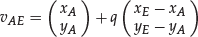
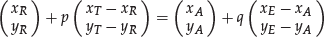
Let current node (i.e., node 8) be denoted by R(x_R,y_R) and the current target node (i.e., node 5) be denoted by T(x_T,y_T). The line pointing from the current node (8) towards the current target node (5), generalized as node T(target) can be represented by the line vector.

v_{R T} = (\begin{matrix} x_{R} \\ y_{R} \end{matrix}) + p (\begin{matrix} x_{T} - x_{R} \\ y_{T} - y_{R} \end{matrix})

(31)

where $(\begin{matrix} x_{T} - x_{R} \\ y_{T} - y_{R} \end{matrix})$ represents the direction of line vector. Similarly, the wall (suppose 6-7 as in figure 7) can be represented by the line vector. Let the wall be denoted by points A(x_A,y_A) and E(x_E,y_E) respectively. The line vector connecting wall AE can thus be represented as:

v_{A E} = (\begin{matrix} x_{A} \\ y_{A} \end{matrix}) + q (\begin{matrix} x_{E} - x_{A} \\ y_{E} - y_{A} \end{matrix})

(32)

Figure 7.

Dijkstra's algorithm: visibility check.

where $(\begin{matrix} x_{E} - x_{A} \\ y_{E} - y_{A} \end{matrix})$ represents the direction vector of the wall. A dot product of the two vectors formed by the path from the current node to the current target node and by the walls/obstacles is used to make sure that the quadrotor path does not intersect with the wall or obstacles. The corresponding intersection point if it exists, is calculated by equating v_RT and v_AE to obtain q. v_RT = v_AE, i.e., the intersection point is common to both vectors

(\begin{matrix} x_{R} \\ y_{R} \end{matrix}) + p (\begin{matrix} x_{T} - x_{R} \\ y_{T} - y_{R} \end{matrix}) = (\begin{matrix} x_{A} \\ y_{A} \end{matrix}) + q (\begin{matrix} x_{E} - x_{A} \\ y_{E} - y_{A} \end{matrix})

(33)

Dissecting the above equation results in two linear simultaneous equations

{\begin{array}{l} x_{R} + p (x_{T} - x_{R}) = x_{A} + q (x_{E} - x_{A}) \\ y_{R} + p (y_{T} - y_{R}) = y_{A} + q (y_{E} - y_{A}) \end{array}

(34)

Solving 34 to express q in terms of p:

{\begin{array}{l} q = \frac{x_{R} - x_{A} + p (x_{T} - x_{R})}{x_{E} - x_{A}} \\ q = \frac{y_{R} - y_{A} + p (y_{T} - y_{R})}{y_{E} - y_{A}} \end{array}

(35)

Substituting 35 into 34 and rearranging we can obtain the p.

p = \frac{(x_{E} - x_{A}) (y_{A} - y_{R}) - (y_{E} - x_{A}) (x_{A} - x_{R})}{(x_{E} - x_{A}) (y_{T} - y_{R}) - (y_{E} - x_{A}) (x_{T} - x_{R})}

(36)

Substituting equation 36 into equation 35 will allow for q to be calculated. In the case of a vertical wall, i.e., x_E − x_A = 0 the first part of equation 34 should be used. Similarly in the case of a horizontal wall, i.e., y_E − y_A = 0, the second part of equation 35 should be used. In the case of non-vertical and non-horizontal walls, either the first part or the second part of equation 35 can be used. The boundary restriction from the quadrotor to the obstacle/wall is also taken into account. The restriction includes the quadrotor dimensional restriction that is from the centre of mass of the quadrotor to its arm end and additional restriction to allow the quadrotor enough space to fly safely in the case of some path deviation. Using a combination of the proposed controller scheme and Dijkstra's algorithm, the quadrotor can find its own optimal path from the given initial position to the final position in an environment with obstacles.

4. Simulation

The simulation of the proposed dynamics, control algorithm and path planning algorithm is performed using the Matlab/Simulink environment. The simulation block of the quadrotor system is as presented in figure 8.

Figure 8.

Matlab/Simulink model of the system.

The task block contains the task or the command for the quadrotor to follow. The task is provided to the Dijkstra algorithm block to compute the optimal path. The optimal path is then provided to the controller block via the command feeder. A total of six controllers are used to fully control the quadrotor. Four of them, namely Z controller, Phi controller, Theta controller and Psi controller, together form the inner loop control and are the basic controllers used to stabilize the quadrotor. It steadies the attitude of the quadrotor while stabilizing the height [11, 15]. The remaining two controllers, the X controller and the Y controller, form the outer loop control. The outer loop control helps to navigate to desired position by providing the desired pitch and desired roll angle for the inner loop control to track down. The wind model available in Simulink library is used to model the wind blowing with a velocity of 1m/s opposite to the X_E axis. The uncertainty on the other hand is imposed on the rotational speed of the motor as described in equation 37

ω_{i} = ω_{i_d e s i r e d} + N (0,10)

(37)

5. Result

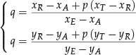
The simulation results of the quadrotor with integrated motor dynamics controlled using a self-tuning fuzzy PID controller, show it to be capable of performing path planning as presented in the figures and tables to follow. Figure 9, 10, 11 and 12 shows the waypoint following performance of the PID controller and the EKF fuzzy PID controller. The initial oscillation on the theta response in figure 11 is the result of the imposed wind model acting opposite to the x axis. Table 1 shows a comparison of performance between the two controllers, where the term “total error” is defined by the sum of the absolute positional error during the whole waypoint following mission. Figure 13 to figure 17 are used to show the performance of the EKF fuzzy PID controller while following the optimal path as calculated from Dijkstra's algorithm. The Matlab simulation (Figure 13), Virtual reality simulation (Figure 14), PID parameter tuning (Figure 15 and figure 16) and fuzzy parameter tuning (Figure 17) are displayed.

Figure 9.

Waypoint following PID.

Figure 10.

Waypoint following EKF fuzzy PID.

Figure 11.

Attitude plot: Waypoint Following: EKF Fuzzy PID.

Figure 12.

Voltage plot (Controlled Input): Waypoint Following: EKF Fuzzy PID.

Figure 13.

Path Planning EKF Fuzzy PID.

Figure 14.

Virtual reality simulation using Matlab/Simulink.

Figure 15.

Tuning of PID gains: Y controller: Path Planning.

Figure 16.

Tuning of PID gains: Phi Controller: Path Planning.

Figure 17.

Fuzzy membership function tuning (at t=85 sec): Path Planning.

Table 1.

Performance comparison table: waypoint following.


Algorithm	Maximum Error [m]	Total Error [m]

PID	0.35	33.6
EKF Fuzzy PID	0.10	9.3

6. Conclusion

The quadrotor was successfully controlled using PID gain scheduling based on an EKF algorithm. The stability control, waypoint following and path planning were successfully simulated. The self-tuning fuzzy PID controller showed good resistance to the induced disturbance and the uncertainty. It adapted to the wind and disturbance quickly and provided significantly better performance as compared to a simple PID controller. The obstacle avoidance and waypoint following performance was enhanced using the self-tuning fuzzy PID controller.

Footnotes

7. Acknowledgment

This work was supported by the 2013 Research Fund of University of Ulsan.

References

Gessow

Myers

(1967) Aerodynamics of the helicopter. Frederick Ungar Publishing Co. New York.

Santos

Lopez

Morata

(2010) Intelligent fuzzy controller of a quadrotor. International Conference on Intelligent Systems and Knowledge Engineering (ISKE). pp.141–146.

Coza

Macnab

C. J. B.

(2006) A New Robust Adaptive-Fuzzy Control Method Applied to Quadrotor Helicopter Stabilization. Annual Meeting of the North American Fuzzy Information Processing Society, pp.454–458.

AI-Younes

Jarrah

M. A.

(2008) Attitude stabilization of quadrotor UAV using Backstepping Fuzzy Logic and Backstepping Least-Mean-Square controllers. International Symposium on Mechatronics and its Applications, pp.1–11.

Amoozgar

M. H.

Chamseddine

Zhang

(2012) Fault-Tolerant Fuzzy Gain-Scheduled PID for a Quadrotor Helicopter Testbed in the Presence of Actuator Faults. IFAC Conference on Advances in PID Control.

Sharma

Barve

(2012) Controlling of Quad-rotor UAV Using PID Controller and Fuzzy Logic Controller. International Journal of Electrical, Electronics and Computer Engineering. 1 (2):38–41.

Sangyam

Laohapiengsak

Chongcharoen

Nilkhamhang

(2012) Path Tracking of UAV Using Self-Tuning PID Controller Based on Fuzzy Logic. SICE Annual Conference, pp.1265–1269.

Szafranski

Czyba

(2011) Different Approaches of PID Control UAV Type Quadrotor. Proceedings of International Micro Air Vehicles Conference. 11.

Altug

Ostrowski

J. P.

Mahony

(2002) Control of a Quadrotor Helicopter Using Visual Feedback. IEEE International Conference on Robotics and Automation. 1:72–77.

10.

Bouabdallah

Siegwart

(2005) Backstepping and Sliding-mode Techniques Applied to an Indoor Micro Quadrotor. IEEE conference on Robotics and Automation. pp.2247–2252.

11.

Tommaso

Bresciani

(2008) Modelling, Identification and Control of a Quadrotor Helicopter. Master Thesis, Lund University, Lund, Sweden.

12.

Ahn

K. K.

Truong

D. Q.

Thanh

T. Q.

Lee

B. R.

(2008) Online self-tuning fuzzy proportional-integral-derivative control for hydraulic load simulator. Institution of Mechanical Engineers Part I Journal of Systems and Control Engineering. 222 (12):81–96.

13.

Ahn

K. K.

Truong

D. Q.

(2009) Online tuning fuzzy PID controller using robust extended Kalman filter. Journal of Process Control. 19 (6):1011–1023.

14.

Dijkstra

E. W.

(1959) A note on Two problems in Connexion with Graphs. Numerische Mathematik. 1:269–271.

15.

Orsag

Poropat

Bogdan

(2010) Hybrid Fly-by-Wire Quadrotor Control. Automatika. 1:19–32.