Sage Journals: Discover world-class research

Abstract

The sky region in an image provides horizontal and background information for autonomous ground robots and is important for vision-based autonomous ground robot navigation. This paper proposes a sky region detection algorithm within a single image based on gradient information and energy function optimization. Unlike most existing methods, the proposed algorithm is applicable to both colour and greyscale images. Firstly, the gradient information of the image is obtained. Then, the optimal segmentation threshold in the gradient domain is calculated according to the energy function optimization and the preliminary sky region is estimated. Finally, a post-processing method is applied in order to refine the preliminary sky region detection result when no sky region appears in the image or when objects extrude from the ground. Experimental results have proven that the detection accuracy is greater than 95% in our test set with 1,000 images, while the processing time is about 150ms for an image with a resolution of 640×480 on a modern laptop using only a single core.

Keywords

Sky Detection Gradient Information Energy Function Optimization Robot Navigation

1. Introduction

The most important problem for autonomous ground robot navigation is the sensing and understanding of the surrounding environment. The most commonly used sensors in autonomous ground robots can be roughly divided into two groups: active sensors and passive sensors. Active sensors such as RADAR, LIDAR and sonar are accurate and popular [1]. With the development of electronics technology, passive sensors such as video cameras can provide abundant information of the environment with a smaller size, lower price and less power consumption. As a result, vision sensors have become increasingly popular in autonomous ground robot navigation [2].

The sky region is an important component for outdoor images and provides information about the environment. The detection of the sky region for outdoor robot navigation is useful [3]. With the detected sky region, the horizon - which is crucial for outdoor robot navigation - can be estimated in the image [4]. In [4], an autonomous ground robot developed by Stanford University was equipped with a colour computer vision system. Using the simple sky region detection algorithm proposed in [16], it could improve the road detection results and estimate the rough tilt angle of the robot. This famous robot was the winner of the DARPA Grand Challenge in 2004. Furthermore, the sky usually belongs to the background and no further image processing techniques are needed in this region such that the computational complexity of the whole vision-based navigation algorithm can be reduced and its robustness can be enhanced. For example, stereo-matching in the sky region is highly unreliable and should be discarded during robot navigation. Figure 1 gives an example. The left image in the figure is the reference image of a stereo pair and the right one is its corresponding disparity image generated by one of the current state-of-the-art stereo matching algorithms [23]. From the figure, we can see that there are many disparity errors in the sky region and that these errors will cause problems to the digital elevation map (DEM) generation and path-planning in robot navigation. However, with our proposed sky region detection algorithm we can eliminate sky region for further consideration and generate a clean DEM (readers can check the sky region detection result of the left image in Figure 1 using our algorithm in the third row of Figure 11). Recently, an interesting algorithm to detect water hazards based on the analysis of the sky region and its reflections was proposed [5]. From the above discussion, we can conclude that sky region detection is closely related to autonomous robot navigation.

Figure 1.

A stereo example captured by the NASA mars rover. The left image is the reference image (the target image is not showed in this figure). The right image is its corresponding disparity image generated by [23]. The brighter pixels stand for a larger disparity value. There are many erroneous disparity values in the region labelled by the red rectangle.

To the best of our knowledge, most of the current sky region detection algorithms depend on the colour information of the image. Vailaya and Jain [6] have proposed to combine colour and texture information to detect the sky region. In their method, the image is divided into square blocks. Colour and texture information is extracted in these blocks. A Bayesian methodology is applied in order to classify square blocks separately without considering neighbourhood relationships. Luo et al. [7] have analysed the dispersion of light rays by small particles in the air according to physics principles and have concluded that the upper part of the sky appears to be blue with high saturation, and that the saturation decreases as the sky gradually attaches the ground. According to this principle, they first estimate the sky region confidence according to colour information through neural networks. They then get the final sky region by combining the gradient and the connected components of the image. Gallagher et al. [8] improved the method in [7] by fitting a 2D polynomial model. Zafarifar et al. [9] have used the hypothesis that the sky is relatively smooth and appears in the upper part of the image. The sky region probability distribution is estimated by combining colour (YUV colour space), position and texture information in the image. They propose a sky region detection algorithm for the application of video image enhancement. They also implemented the algorithm on FPGA and achieved a speed of 30fps [10]. McGee et al. [11] converted the image into a YCrCb colour space and classified the sky region with SVM in order to detect obstacles in the air. Laungrugthip et al. [12] have made use of edge information in the blue channel of the colour image together with morphological operations and have proposed a simple sky region detection method for solar exposure prediction. Rankin et al. [5] have proposed a rule-based sky detection method by analysing the saturation-to-brightness ratio, monochrome intensity variance and edge magnitude. The horizon position in the image, which is estimated from the inertial sensors of the robot, is also included in order to restrict the sky search region and improve the robustness of the algorithm. This method can classify different types of sky, such as overcast, clear and cloudy. All these proposed methods need colour information from the image, which restricts the application of these algorithms.

Recently, object/region detection algorithms have gradually matured. Most of these methods rely on the multi-scale sliding window technique [24,25]. As a result, the detection results are usually represented by coarse bounding boxes, which are obviously not accurate enough for the complex shapes of sky regions. Image segmentation also has a long history and there are several successful methods [26,27]. However these techniques mainly concentrate on low-level features in the image and ignore semantic meanings. As a result, semantic regions (such as the sky region) in the images usually break into small parts using these methods. Semantic segmentation algorithms have made great progress over these years. Some of them can detect sky regions in the image [13 –15,28]. However, these algorithms are general purpose detection algorithms and are not designed specifically for sky regions. Thus, their accuracy is highly dependent on the objects' interactions in the image. Usually, the detection accuracy of this kind of algorithm is around 80%, which is not very accurate [13,28]. Furthermore, the computational complexity of these algorithms is usually very high due to the complex feature extraction and pattern classification steps. The training time is in the order of tens of hours, and the testing time is usually several seconds on a modern high-end PC [13]. As a result, it prohibits their application in autonomous ground robot navigation. On the contrary, our proposed method does not need training and the testing time is much faster.

Ettinger et al. [16] propose a horizon detection algorithm. They simplify the border between the sky and the ground as a straight line and get the optimal border line according to energy function maximization with 2D search technology based on image pyramids. This algorithm can be applied to both colour images and greyscale images. Unfortunately, the border line is simplified as a straight line, which is not sufficiently accurate when the border between the sky and the ground is complex. This method was applied to the famous Stanford autonomous ground robot ‘Stanley’ for estimating the tilt angle of the vehicle [4].

Figure 2.

Two examples of images with sky regions. Notice that the sky regions are not blue in these images.

In many situations, the sky region does not appear to be blue. The sense of blue is a complex combination of light optics and the prior knowledge of human beings. However, the size of the particles in the air varies according to the weather conditions. Furthermore, there is no subjective effect such as prior knowledge or visual processing by the human brain for digital cameras. As a result, sky regions in digital images are not always blue. Figure 2 gives two examples in which the sky regions are not blue. In considering the application of vision-based ground robot navigation, we propose an efficient sky region detection algorithm in this paper based on the following assumptions:

The luminance of the sky region changes smoothly.

The application is in autonomous ground robot navigation, and so we assume that the sky region is above the ground region.

With the above assumptions, a sky region detection algorithm based on a single image is proposed. Firstly, gradient information is obtained from the image. With the gradient information, the image is divided into sky and ground regions according to energy function maximization. Finally, a post-processing technique is applied in order to detect images without sky regions and objects extruding from the ground so that the sky region can be detected precisely. The proposed algorithm can track the border between the sky and the ground precisely and the computational complexity is acceptable. It is suitable for those applications that are time critical or else employ restricted computational resources, such as autonomous land vehicle (ALV) and planet rover (the mars rover, the lunar rover, etc.) navigation. Figure 3 gives the flow chart of the whole algorithm.

Figure 3.

Flow chart of the proposed algorithm.

2. Algorithm Details

2.1 Image Pre-processing and Gradient Image Calculation

If the input image is a colour image, we convert it into a greyscale image. From the greyscale image, we calculate its corresponding gradient image with the Sobel operator [17]. As is known, the Sobel operator contains two operators in the horizontal and vertical directions. We convolve the input greyscale image with these two operators and get two gradient images. Finally we calculate the gradient magnitude image by combining the two gradient images. Figure 4 shows an example of the gradient magnitude image (the image is normalized for viewing purposes). The gradient magnitude image is applied in energy function optimization, as described in section 2.2.2.

Figure 4.

The gradient magnitude image which corresponds to the left image in Figure 2.

2.2 Preliminary Sky Region Detection

2.2.1 Definition of the Energy Function

Inspired by the energy function proposed in [16], we make certain modifications and define an energy function suitable for our applications. In [16], the original colour image is divided into sky and ground regions. The pixels in both regions are denoted by their RGB components. The energy function defined in [16] is as follows:

J = \frac{1}{| Σ_{s} | + | Σ_{g} | + {(λ_{1}^{s} + λ_{2}^{s} + λ_{3}^{s})}^{2} + {(λ_{1}^{g} + λ_{2}^{g} + λ_{3}^{g})}^{2}}

(1)

where Σ_s and Σ_g are the covariance matrices of the pixels that are described by RGB values in sky and ground regions, respectively. They are both 3×3 matrices, which are defined as follows:

Σ_{s} = \frac{1}{N_{s}} \sum_{(y, x) \in s k y} (I^{s} (y, x) - μ^{s}) {(I^{s} (y, x) - μ^{s})}^{T}

(2)

Σ_{g} = \frac{1}{N_{g}} \sum_{(y, x) \in g r o u n d} (I^{g} (y, x) - μ^{g}) {(I^{g} (y, x) - μ^{g})}^{T}

(3)

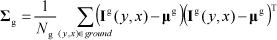
where N_s and N_g are the number of pixels in the sky and ground regions, respectively, while µ^s and µ^g are 3×1 column vectors that represent the average RGB values in the sky and ground regions, respectively.

λ^s_i and λ^g_i (i = {1, 2, 3}) are Eigen values corresponding to the above two matrices and |·| denotes the determinant, that measures the variance or volume of the pixel distribution in each region. In equation (1), the square of the sum of the Eigen values is introduced in order to cope with those conditions under which the video frames lose colour information, so that the determinants of both matrices become singular. It is obvious that maximizing equation (1) can minimize the intra-class variance of the ground and sky distributions.

In our applications, the algorithm has as its main purpose autonomous ground robot navigation. According to assumption 1 in section 1, we emphasize the coherence in the sky region. When video frames lose colour information or the image is a greyscale image, the determinants of both matrices become singular and the ranks of both matrices are almost 1. From matrix theory, we have:

| Σ | = λ_{1} \cdot λ_{2} \cdot λ_{3} \approx 0

(4)

As a result, their corresponding Eigen values satisfy the following formula:

| λ_{1} | > > | λ_{2} | \approx | λ_{3} | \approx 0

(5)

So, with the original colour or greyscale image, our modified energy function is as follows:¹

J_{n} = \frac{1}{γ \cdot | Σ_{s} | + | Σ_{g} | + γ \cdot | λ_{1}^{s} | + | λ_{1}^{g} |}

(6)

where γ denotes our emphasis on the homogeneity in the sky region. In this paper, we choose γ = 2 experimentally. Since |λ₂| and |λ₃| are very small compared with the largest Eigen value |λ₁| of the matrix when the matrix is nearly singular, we omit the terms λ₂ and λ₃ in equation (6).

2.2.2 Energy Function Optimization

According to the energy function defined in the previous section, we can get the optimal sky and ground regions segmentation result by optimizing the energy function. In order to optimize the energy function, its parameters have to be defined.

In [16], the energy function is parameterized by a bank angle and a pitch value, which represent a straight line in the image. As mentioned in section 1, a simple straight line is not enough for the application of autonomous ground robot navigation. Furthermore, the computational complexity of the 2D parameters' space search is still quite high, even with the help of the image pyramids technique. Unlike the method in [16], a novel parameterization strategy with only one parameter is proposed in this paper.

Firstly, we define a sky border position function b(x):

1 \leq b (x) \leq H (1 \leq x \leq W)

(7)

where W and H are the width and height of the image, respectively, and b(x) determines the sky border position in the x^th column. That is to say, the sky and ground regions can be calculated with the following equations:

s k y = {(x, y) | 1 \leq x \leq W, 1 \leq y \leq b (x)}

(8)

g r o u n d = {(x, y) | 1 \leq x \leq W, b (x) < y \leq H}

(9)

We use a parameter t, which is a threshold, to calculate the sky border position function b(x) so that the sky and ground regions can be further calculated according to equations (8) and (9). The following pseudo-codes show the algorithm for calculating the sky border position function b(x) from parameter t.

Figure 5.

A typical plot of J_n(t).

Algorithm 1. Calculate sky border position function:

Calculate_border(grad, t).

Input: threshold t; gradient image grad.

Output: sky border position function b(x).

for x = 1 to W b(x) = H for y = 1 to H if grad(y,x) > t b(x) = y break end if end for end for

Algorithm 2. Energy function optimization algorithm.

Input: Search space of t∈[thresh_min, thresh_max]; number of sample points n in the search space; gradient image grad.

Output: The optimal sky border position function b_opt(x).

Initialize b_opt = Ø, b_tmp = Ø, J_n__max = 0 for k = 1 to n

t = t h r e s h_m i n + \frac{t h r e s h_m a x - t h r e s h_m i n}{n - 1} \times (k - 1)

b_tmp = Calculate_border(grad, t) Calculate J_n(t) with its corresponding b_tmp. if J_n(t) > J_n__max J_{n_max} = J_n(t) b_opt = b_tmp end if end for

For a given threshold t, we can get b(x) according to algorithm 1. Combining equations (8) and (9), the sky and ground segmentation result corresponding to t can be calculated and J_n(t) can be estimated without difficulty. As shown in Figure 5, the relationship between t and J_n(t) is quite complex and nonlinear. Thus, it is difficult to optimize J_n(t) globally with the traditional gradient-based method. Fortunately, our proposed energy function J_n(t) only depends on a single parameter t, and it is feasible to optimize it by searching in a 1D parameter space, which is shown as pseudo-codes in algorithm 2.

With the optimal sky border position function b_opt(x) calculated from algorithm 2, its corresponding optimal sky and ground segmentation result can be calculated according to equations (8) and (9). In algorithm 2, there are several parameters that need to be determined. They are: thresh_min, thresh_max and n. According to the definition of the Sobel operator, the maximum value in the gradient image is about 1,443 for a traditional 8-bit greyscale image. In theory, we have: thresh_min > 0 and thresh_max = 1443. But, as we looked at Figure 5 and analyse it in detail, we found that for a natural image it is unlikely that the intensity difference between the neighbouring pixels will reach 255. As a result, the maximum value of the gradient image should not be expected to reach 1,443. From Figure 5, we can also see that if the threshold t exceeds 600, J_n(t) is nearly a constant. Considering the balance between search precision and computational complexity, we set the sampling step in the search space of t as search_step = 5, so that:

t h r e s h_m i n = 5, t h r e s h_m a x = 600

(10)

n = \frac{t h r e s h_m a x - t h r e s h_m i n}{s e a r c h_s t e p} + 1 = \frac{600 - 5}{5} + 1 = 120

(11)

Figure 6 shows the preliminary sky region detection result of the left image in Figure 2. We can see that the sky border can be detected precisely.

Figure 6.

Preliminary sky region detection result. In the left image, the black curve is the sky border. In the right image, the black region is the sky region and the rest is the ground region.

2.3 Sky Region Refinement and Post-processing

2.3.1 Detection of the Image without a Sky Region

Sometimes, there is no sky region in an image. Unfortunately, the method proposed in the previous sections assumes that there are sky regions in the image and aims to detect them. As such, there will be some fake sky regions in those images with no sky region when applying the previously proposed method. In this section, we propose a method to overcome these drawbacks.

Figure 7.

Two examples of images without a sky region. Fake sky regions are extracted by the algorithm proposed in section 2.1 and 2.2. The left column shows the sky borders in black dots and the right column shows the corresponding sky regions in black areas.

Figure 7 shows two typical sky region detection results. In both images, there are no sky regions but the previously proposed method detects fake sky regions. In the first row of Figure 7, there are highly textured trees in the image and the gradient values are large all over the image. Accordingly, the sky border position function is near the upper border of the image. The second row of Figure 7 is captured by the Mars Exploration Rover (MER) Spirit, launched by NASA [18]. This image contains sand-like ground and many rocks of different sizes. The gradient values are relatively small in this image and the sky border position function varies in a wide range with the different positions of the rocks in each column. From the analysis above, we arrive at the conclusion that the fake sky regions in images without sky have the following properties:

The sky border position function is near the upper border of the image. That is to say: the sky region only occupies a small portion of the image.

The sky border appears in a “zigzag” shape. That is to say: the sky border position function jumps rapidly in a wide range.

For the first case, we define the average of the sky border position function:

b o r d e r_a v e = \frac{1}{W} \sum_{x = 1}^{W} b (x)

(12)

If border_ave is less than a predefined threshold, this means that the detected sky region only occupies a very small part of the image. This image does not contain a sky region.

For the second case, we define the average of the sum of absolute differences of the sky border positions (ASADSBP) as follows:

A S A D S B P = \frac{1}{W - 1} \sum_{x = 2}^{W} | b (x) - b (x - 1) |

(13)

A large ASADSBP means frequent changes in the sky border position function. Combining the above two cases, we can draw the conclusion that if the following equation is satisfied, there is no sky region in the image.

(border_ave < thres h_{1}) \lor (b o r d e r_a v e < t h r e s h_{2} \land A S A D S B P > t h r e s h_{3})

(14)

In equation (14), there are three threshold values:thresh₁, thresh₂ and thresh_3. They are determined according to experiments. In this paper, we set them to be the following values:

t h r e s h_{1} = H / 30, t h r e s h_{2} = H / 10, t h r e s h_{3} = 5

(15)

2.3.2 Detection and Refinement of the Image Columns without a Sky Region

During the image capture process, sometimes the camera is slanted or there are tall objects in the scene; there might be some image columns which do not contain a sky region. As shown in Figure 8, there are fake sky regions detected in the middle of the image while directly applying the previous proposed algorithm. The reason is that our proposed algorithm implicitly assumes that there are sky region pixels in every column.

In order to overcome this drawback, we have to first detect it. Observing that there is a sudden change of sky border positions in Figure 8, we define the absolute differences of sky border positions:

d i f f_a b s (x) = | b (x + 1) - b (x) | (1 \leq x \leq W - 1)

(16)

If the following equation is satisfied, we believe that there are image columns which do not contain a sky region:

d i f f_a b s (x) > t h r e s h_{4} (\exists x \in [1, W - 1])

(17)

We find that thresh₄ = H/3 can produce a satisfactory result.

Figure 8.

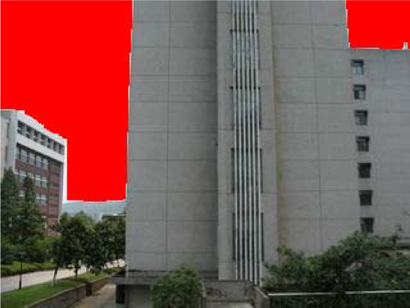
Sky region detection results of an image with some columns that do not contain a sky region. The left image shows the detected sky border in red lines. The right image shows the corresponding sky region painted in red.

As soon as we have detected the presence of a fake sky region in some image columns, we need to separate them from the true sky region. Since the fake sky region is actually an object on the ground, they are assumed to have a different appearance from any sky regions. We apply the K-means algorithm [19] to separate the sky region into two clusters. Each pixel is described in a RGB colour space (A greyscale image can also be described in a RGB colour space by setting the red, green and blue channels to the same value.). We can get mean vectors µ^s1 and µ^s2, and covariance matrices Σ_s1 and Σ_s2 of the two clusters. We also calculate the mean vector µ^g and the covariance matrix Σ_g corresponding to the ground region. We calculate the Mahalanobis distances between µ^s1 and µ^g, µ^s2 and µ^g. We compare them and set the cluster with the larger distance as the sky region cluster. Its corresponding mean vector and covariance matrix are µ^s_true and Σ^s_true, respectively.

In order to refine the sky border positions, we need to recalculate b(x). The pseudo-codes of the algorithm are as follows.

Algorithm 3. Sky border position function recalculation algorithm.

Input: µ^s_true, Σ_{s_true}, µ^g, Σ^g, original sky border position function b(x), original image I.

Output: Recalculated sky border position function b_new(x).

Initialize: cnt = 0 for x = 1 to W for y = 1 to b(x)

Calculate the Mahalanobis distance between every pixel from the original sky region and the refined sky region cluster centre:

d i s t_s = {(I^{s} (y, x) - μ^{s_true})}^{T} \sum_{s_true}^{- 1} (I^{s} (y, x) - μ^{s_true})

Calculate the Mahalanobis distance between every pixel from the original sky region and the ground region cluster centre:

d i s t_s = {(I^{s} (y, x) - μ^{g})}^{T} \sum_{g}^{- 1} (I^{s} (y, x) - μ^{g})

if dist_s <dist_g cnt = cnt + 1 end if end for if $c n t < \frac{b (x)}{2}$ b_new(x) = 0 else b_new(x) = b(x) end if end for

Figure 9.

Refined sky region for Figure 8. The sky region is labelled in red.

When the image is a greyscale image, we have rank (Σ_{s_true}) = rank(Σ_g) = 1, and the inverse matrices are ill-posed when calculating the Mahalanobis distances. We use the reciprocal of any diagonal element in the matrix instead. Figure 9 shows the refined sky region of Figure 8. The sky region is correctly detected.

2.4 Summary of the Whole Algorithm

For the sake of completeness and the clarification of the whole procedure of our proposed algorithm, we present pseudo-codes of our algorithm as follows.

Algorithm 4. Sky region detection algorithm.

Input: original image I for sky region detection.

Output: detected sky region.

Calculate the gradient image grad according to section 2.1.

Calculate the optimal sky border position function b_opt(x) with algorithm 2.

Calculate border_ave and ASADSBP according to equations (12) and (13).

Test border_ave and ASADSBP according to equation (14).

if equation ( 14 ) is satisfied There is no sky region in the image. return else Calculate diff_abs(x) according to equation ( 16 ). Test diff_abs(x) according to equation ( 17 ). if equation ( 17 ) is satisfied Recalculated the sky border position function b_new(x) with algorithm 3. Calculate the sky region with b_new(x) according to equation ( 8 ). return else Calculate the sky region with b_opt(x) according to equation ( 8 ). return end if end if

Figure 10.

Comparison of sky region detection results. The leftmost column is the original image; the second column is the result of our proposed algorithm; the third column is the result by [5]; the rightmost column is the result by [16]. The first three images are from MSRC (twenty-three class subset); the fourth image is from OSU-ACT Urban Scene sequences; the last two images are from our own image collection.

3. Experimental Results

3.1 Dataset Organization

To the best of our knowledge, there is no suitable benchmark dataset for evaluating sky region segmentation accuracy. As a result, we organize our own dataset instead. Our dataset includes 1,000 images and contains both colour and greyscale images. This dataset consists of four subparts. The details about each subpart of the dataset are as follows:

MSRC (twenty-three class subset): This image set is constructed by Shotton et al. from Microsoft Research, Cambridge [20]. The original purpose of this dataset is to serve as a benchmark for object class recognition. Since it contains a sky class, we adopt this dataset. However, since our proposed algorithm is applied to outdoor autonomous ground robots, we eliminate images which contain indoor scenes, specific traffic signs and very large areas of bodies of water. As a result, we only maintain a subset of the original dataset. This subset contains 360 images. They are all colour images with a resolution of 320×213.

OSU-ACT Urban Scene sequences: This subset is captured by a low cost digital camera on the roof of the ACT autonomous ground robot from the Ohio State University [21]. It recorded the scene when ACT was driving around the campus of the Ohio State University at Columbus, OH. This subset contains 200 images. They are all low quality colour images with a resolution of 640×480.

NASA mars rover subset: This subset was captured by the navigation cameras of the two mars rovers Spirit and Opportunity, launched by NASA in 2004. The images were all captured on the surface of Mars [22]. This subset contains 200 images. They are all greyscale images with a resolution of 1024×1024.

Our own image collection: This subset was captured by a Canon PowerShot A630 digital camera. The images were collected for different outdoor scenes. There are 120 colour images and 120 greyscale ones. All the images are 640×480.

Our test dataset contains a wide variety of different outdoor scenes. Some examples are shown in the left columns of Figure 10 and Figure 11.

3.2 Qualitative and Quantitative Results

We choose to compare our algorithm against the algorithms proposed in [5] and [16]. All the codes are implemented in C++ by ourselves. The parameters needed in the algorithms proposed in [5] and [16] are set by maximizing the performances in our test dataset. The reason for choosing [5] is that it was designed specifically for autonomous ground robots and was published in a recent world premier robotics conference. The method in [16] is one of the very few algorithms that can be applied to both colour and greyscale images, and was published in a mainstream conference.

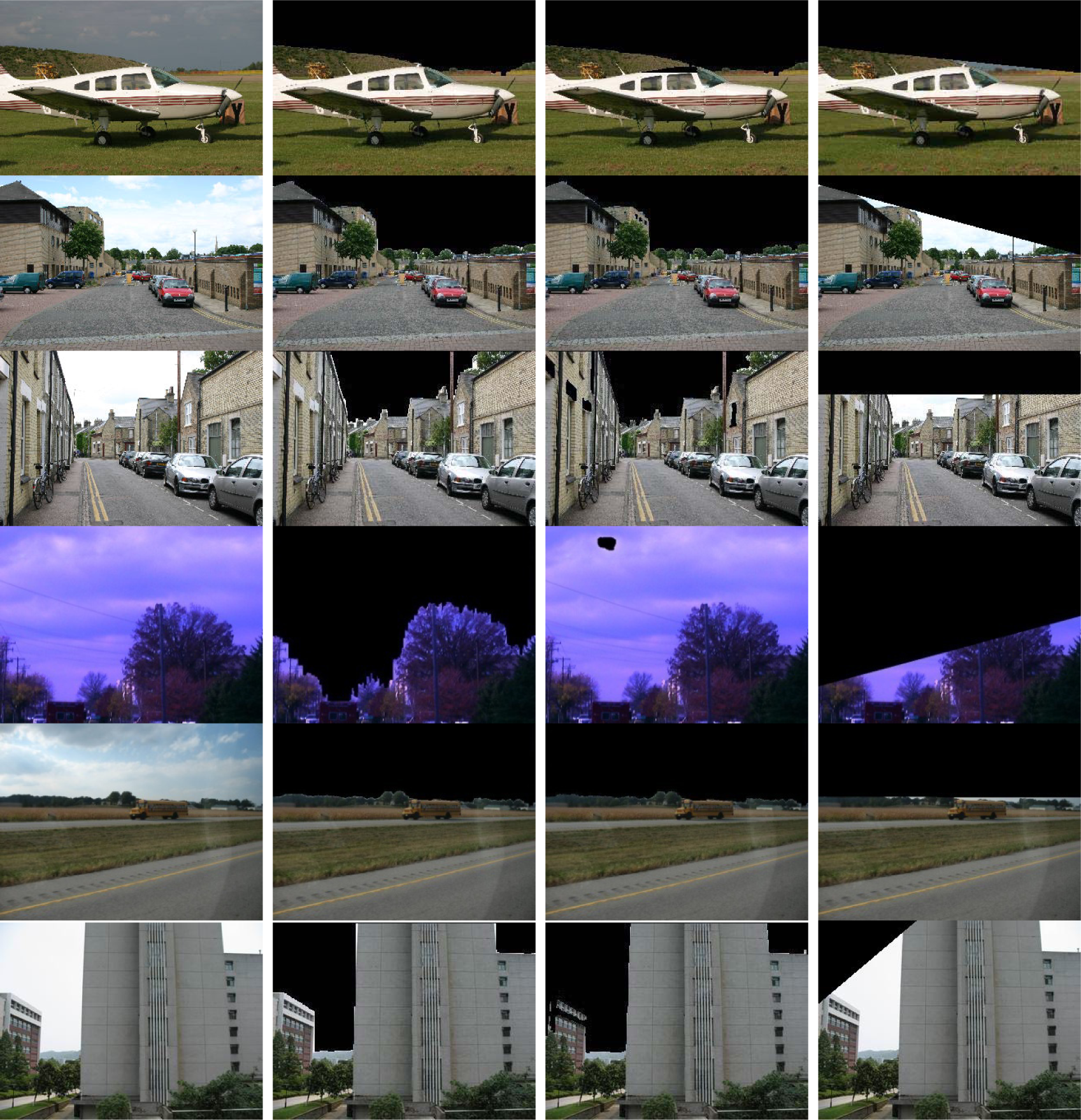
Since the algorithm proposed in [5] can only be applied to colour images, we only test it using the 680 colour images in our dataset. Furthermore, the algorithm proposed in [5] needs readings from inertial sensors, which are not provided in our dataset, to estimate horizon lines in images. In order to make a fair comparison, we label the horizon lines manually to serve as an input to the algorithm proposed in [5]. The results are shown in Figure 10. In this figure, we can see that our proposed algorithm performs well. The clouds in the second, fourth and fifth images do not cause any problems for our proposed algorithm. This proves that our smooth transition assumption in the sky region is valid. On the other hand, the algorithm proposed in [5] does not perform very well. That method depends on the analysis of the appearance of every single pixel. As a result, bright regions above horizon line can be easily misclassified as a sky region. This can be seen in the first, third and last images. In the first image, part of the white roof of the airplane is misclassified as a sky region. In the third image, the white walls above the windows in the left part and the bright window near the middle part are all misclassified as sky regions. In the last image, the white walls of the buildings that connect with the sky region are also erroneously classified as sky regions. The fourth image is captured by a low cost digital camera and the colour shifts heavily towards violet. This causes difficulties for the algorithm proposed in [5], which is rule-based and could not detect the abnormal “violet sky”. Instead, only a small region of white clouds is detected as sky.

We compare our proposed method against the algorithm proposed in [16] on our full test dataset. The results can be found in Figure 10 and Figure 11. In all the images of Figure 11, sky regions are detected reliably by our algorithm. In the second row, the sky region is quite dark. In the fifth row, the border between the sky and the ground is not obvious and the brightness in the sky region spans quite a large range. None of these difficulties cause any problems to the detection results for our proposed algorithm. However, the simplified line border of the algorithm proposed in [16] can hardly capture the complex borders between the sky and the ground in most of the images in Figure 10 and Figure 11.

In order to analyse the results quantitatively, we compare the results against benchmark sky regions in our test dataset. The twenty-three class subset of MSRC is companioned with ground truth sky segmentation results. For the remaining 640 images, we manually label the sky regions as benchmarks. Figure 12 shows two of the manually labelled images. We calculate the sky region pixels set sky_bench and the ground region pixels set ground_bench in the benchmark images. During the quantitative analysis step, we calculate the common sky region pixels set and common ground region pixels set:

s k y_{c o m m o n} = {(x, y) | (x, y) \in s k y \land (x, y) \in s k y_{b e n c h} \land 1 \leq x \leq W \land 1 \leq y \leq H}

(18)

g r o u n d_{c o m m o n} = {(x, y) | (x, y) \in g r o u n d \land (x, y) \in g r o u n d_{b e n c h} \land 1 \leq x \leq W \land 1 \leq y \leq H}

(19)

We define the sky region detection precision, ground region detection precision and whole image segmentation precision as follows:

\begin{matrix} P_{s} = \frac{| s k y_{common} |}{| s k y_{bench} |} \times 100 % & P_{g} = \frac{| g r o u n d_{common} |}{| g r o u n d_{bench} |} \times 100 % \end{matrix}

(20)

P_{t} = \frac{P_{s} \cdot | s k y_{bench} | + P_{g} \cdot | g r o u n d_{bench} |}{| s k y_{bench} | + | g r o u n d_{bench} |} \times 100 %

(21)

Table 1.

Quantitative comparison between our proposed algorithm and the algorithm proposed in [5] with colour images in our test dataset.

	Our proposed algorithm			Algorithm proposed in [5]
	P_s(%)	P_g(%)	P_t(%)	P_s(%)	P_g(%)	P_t(%)
Mean value	96.47	96.94	96.81	90.64	86.57	89.23
Standard deviation	1.22	1.67	0.59	5.74	8.24	5.18

Figure 11.

Comparison of the sky region detection results. The left column is the original image, the centre column is the result of our proposed algorithm, and the right column is the result of [16]. The first five images are from the NASA mars rover subset. The last image is from our own image collection.

Figure 12.

Samples of manually labelled sky regions. The sky regions are in black.

Table 1 shows the results on 680 colour images of our proposed algorithm and the algorithm proposed in [5]. From the table, we can conclude that the detection accuracy of [5] is lower than our proposed algorithm, even though it is provided with extra horizon line information. Table 2 shows the results on the whole database with our proposed algorithm and the algorithm proposed in [16]. From the table, we see that the detection accuracy of [16] is much lower than our proposed algorithm and that the detection accuracy is not consistent among the images.

Table 2.

Quantitative comparison between our proposed algorithm and the algorithm proposed in [16] with the whole test dataset.

	Our proposed algorithm			Algorithm proposed in [16]
	P_s(%)	P_g(%)	P_t(%)	P_s(%)	P_g(%)	P_t(%)
Mean value	96.29	95.98	96.05	75.80	80.63	77.44
Standard deviation	1.25	1.70	0.62	27.28	24.01	23.11

We would also like to mention that our proposed method aims at dealing with relatively simple and smooth sky region borders. For those very complex and intricate sky borders, our method can only provide a rough outline of the border (readers might look at the silhouettes of the trees in Figure 10 and Figure 11). However, for the application of robot navigation, the accuracy of our method is enough.

3.3 Parameters Selection and Analysis

In this section, we discuss how to select several parameters used in our proposed algorithm. These parameters are: γ in equation (6), thresh₂ and thresh₃ in equation (14) and thresh₄ in equation (17). Since the physical meaning of thresh₁ is very clear, it could easily be pre-defined explicitly. We do not discuss thresh₁ in this section.

In order to determine the above mentioned parameters, we collect three extra training sets that are different from the dataset described in section 3.1. All these training sets are colour images captured by our Canon PowerShot A630 digital camera. All the images are 640×480. The first training set train₁ contains 100 images. Every image in train₁ has normal continuous sky regions. That is to say, for every column of the image, there exist sky region pixels. The second training set train₂ contains 100 images. None of the images in train₂ has a sky region. The third training set train₃ also contains 100 images. All the images in train₃ have separated sky regions similar to Figure 8. That is to say, for every image in this set, there exist some columns which do not contain any sky region pixels. We also labelled benchmark sky regions manually for all the images.

We first describe how to choose γ. We only apply train₁ for this purpose. This is because, while using train₁, we only need to apply Algorithm 2 in order to detect the sky region, and no other parameters such as thresh₁ to thresh₄ are involved. Figure 13 demonstrated the whole range of image segmentation precisions defined in equation (21) with different choices of γ.

Figure 13.

Whole image segmentation precisions versus different choices of γ.

From Figure 13, we can conclude that the accuracy is high when γ is between 2 and 6. In order to prevent the problem of data overflow, it is better to choose a relatively small value. So, we set γ = 2.

Next, we describe how to determine thresh₂ and thresh₃ simultaneously. This time, we use the full training sets train₁, train₂ and train₃. Since thresh₂ and thresh₃ are used in equation (14) in order to classify whether there exist sky regions or not, we estimate the classification accuracy instead of whole image segmentation precisions described previously. This time, we set γ = 2. Figure 14 shows the result.

Figure 14.

Sky region existence detection accuracy versus different choices of thresh₂/H and thresh₃.

From this figure, we can conclude that the values around thresh₂ = H/10, thresh₃ = 5 can produce satisfactory results.

Finally, we discuss how to choose thresh₄. Since thresh₄ is applied in equation (17) in order to classify whether the image has disrupted sky borders, we again calculate the classification accuracy instead of the whole image segmentation precisions. This time, we use the training sets train₁ and train₃ instead of the whole training sets. This is because train₂ includes images without sky regions such that they will not be passed to the evaluation of equation (17). The results can be found in Figure 15.

Figure 15.

Detection accuracy versus different choices of thresh₄/H.

From this figure we can conclude that the detection accuracy is not very sensitive to the different choices of thresh₄. The accuracy is acceptable for thresh₄ between H/5 and H/2. As a result, we simply choose an approximate mid-value thresh₄ = H/3 in this paper.

3.4 Computational Complexity Analysis

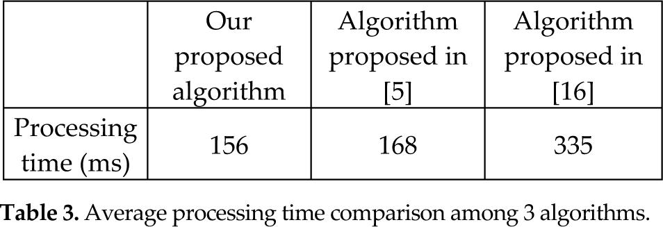
We implemented all three algorithms with unoptimized C++ and test them on a laptop equipped with an Intel P7350 2.0GHz CPU and 2GB RAM. The average processing time of a colour image with a resolution 640×480 is demonstrated in Table 3. From this table, we can conclude that our algorithm is the most efficient. This proves the superiority of our proposed algorithm. It is worth pointing out that our codes only use a single core on the CPU and the proposed energy function optimization algorithm can be easily parallelized and accelerated. For an image with a higher resolution, we can detect a rough sky region in a low resolution and then calculate the accurate sky border in the high resolution image with the image pyramid technique.

Table 3.

Average processing time comparison among 3 algorithms.

	Our proposed algorithm	Algorithm proposed in [5]	Algorithm proposed in [16]
Processing time (ms)	156	168	335

4. Conclusions

This paper proposes a sky region detection algorithm based on a single image. The algorithm mainly applied the prior knowledge that the brightness of a sky region changes smoothly. This assumption is relatively weak, so that our algorithm can be applied to both colour and greyscale images. Quantitative and qualitative experimental results showed that our algorithm is robust compared with the existing algorithms and that the computational cost is relatively low. In the future, we plan to add texture information in order to improve the performance in more complicated scenarios.

Footnotes

17. Acknowledgments

The first author would like to thank Professor Umit Ozguner for providing the urban video sequences test set captured by the OSU-ACT autonomous vehicle platform while the first author was a visiting scholar at the Department of Electrical and Computer Engineering, Ohio State University. The first author was partially supported by the Science and Technology Department of Jiangsu Province (BY2012125). The second author was supported by the National Science Foundation of China (61001143).

1

In theory, maximizing equation () is equivalent to minimizing its denominator. However, occasionally the denominator is very large (in the order of 10¹⁰), so it is safer to maximize equation (6) during the algorithm's implementation to cope with the data overflow problem.

References

Urmson

Ragusa

Ray

Anhalt

Bartz

Galatali

Gutierrez

Johnston

Harbaugh

Kato

Messner

Miller

Peterson

Smith

Snider

Spiker

Ziglar

Whittaker

Clark

Koon

Mosher

Struble

, (2006) A Robust Approach to High-Speed Navigation for Unrehearsed Desert Terrain. J. field robot. 23: 467–508.

Matthies

Maimone

Johnson

Cheng

Willson

Villalpando

Goldberg

Huertas

, (2007) Computer Vision on Mars. Int. j. comput. vision. 75: 67–92.

Kim

Trinh

, (2007) Regions Segmentation Using Multiple Cues for Robot Navigation on Outdoor Environment. International Conference on Control, Automation and Systems. 1768–1772.

Thrun

Montemerlo

Dahlkamp

Stavens

Aron

Diebel

Fong

Gale

Halpenny

Hoffmann

Lau

Oakley

Palatucci

Pratt

Stang

Strohband

Dupont

Jendrossek

Koelen

Markey

Rummel

Niekerk

Jensen

Alessandrini

Bradski

Davies

Ettinger

Daehler

Nefian

Mahoney

, (2006) Stanley: The Robot that Won the DARPA Grand Challenge. J. field robot. 23: 661–692.

Rankin

Matthies

Bellutta

, (2011) Daytime Water Detection Based on Sky Reflections. International Conference on Robotics and Automation. 5329–5336.

Vailaya

Jain

, (2000) Detecting Sky and Vegetation in Outdoor Images. IS&T/SPIE Conference on Storage and Retrieval for Media Databases. 411–420.

Luo

Etz

, (2002) A Physical Model-Based Approach to Detecting Sky in Photographic Images. IEEE trans. image process. 11: 201–212.

Gallagher

Luo

Hao

, (2004) Improved Blue Sky Detection Using Polynomial Model Fit. International Conference on Image Processing. 2367–2370.

Zafarifar

With

, (2006) Blue Sky Detection for Picture Quality Enhancement. The 8th International Conference on Advanced Concepts for Intelligent Vision Systems. 522–532.

10.

Quach

Zafarifar

Gaydadjiev

, (2007) Real-time FPGA-Implementation for Blue-Sky Detection. IEEE International Conference on Application-Specific Systems, Architectures and Processors. 76–82.

11.

McGee

Senqupta

Hedrick

, (2005) Obstacle Detection for Small Autonomous Aircraft Using Sky Segmentation. International Conference on Robotics and Automation. 4679–4684.

12.

Laungrungthip

McKinnon

Churcher

Unsworth

, (2008) Sky Detection in Images for Solar Exposure Prediction. New Zealand Computer Science Research Student Conference. 78–83.

13.

Shotton

Winn

Rother

Criminisi

, (2009) Textonboost for Image Understanding: Multi-Class Object Recognition and Segmentation by Jointly Modeling Appearance, Shape and Context. Int. j. comput. vision. 81: 2–23.

14.

Bergman

Nachlieli

, (2011) Perceptual Segmentation: Combining Image Segmentation with Object Tagging. IEEE trans. image process. 20: 1668–1681.

15.

Gould

, (2012) Multiclass Pixel Labeling with Non-Local Matching Constraints. IEEE Conference on Computer Vision and Pattern Recognition. 2783–2790.

16.

Ettinger

Nechyba

Ifju

Waszak

, (2002) Vision-Guided Flight Stability and Control for Micro Air Vehicles. International Conference on Intelligent Robots and Systems. 2134–2140.

17.

Gonzales

Woods

, (2008) Digital Image Processing. Upper Saddle River: Prentice-Hall Press.

18.

Maki

Bell

Herkenhoff

Squyres

Kiely

Klimesh

Schwochert

Litwin

Willson

Johnson

Maimone

Baumgartner

Collins

Wadsworth

Elliot

Dingizian

Brown

Hagerott

Scherr

Deen

Alexander

Lorre

, (2003) Mars Exploration Rover Engineering Cameras. J. geophys. res. 108: 8071–8094.

19.

Lloyd

, (1982) Least Squares Quantization in PCM. IEEE trans. inf. theory. 28: 129–137.

20.

Microsoft Research Cambridge (2012) Microsoft Research Cambridge 23 Object Classes Database. Available: http://research.microsoft.com/en-us/projects/objectclassrecognition/default.aspx. Accessed 2012 Sep 16.

21.

Ozguner

, (2008) A History of AHS at OSU and Future Progress. IEEE International Conference on Vehicular Electronics and Safety. 13–15.

22.

NASA (2012) MER Analyst's Notebook. Available: http://anserver1.eprsl.wustl.edu/. Accessed 2012 Sep 16.

23.

Hirschmuller

, (2008) Stereo Processing by Semiglobal Matching and Mutual Information. IEEE trans. pattern anal. mach. intell. 30: 328–341.

24.

Dalal

Triggs

, (2005) Histograms of Oriented Gradients for Human Detection. IEEE Conference on Computer Vision and Pattern Recognition. 886–893.

25.

Lampert

Blaschko

Hofmann

, (2008) Beyond Sliding Windows: Object Localization by Efficient Subwindow Search. IEEE Conference on Computer Vision and Pattern Recognition. 1–8.

26.

Shi

Malik

, (2000) Normalized Cuts and Image Segmentation. IEEE trans. pattern anal. mach. intell. 22: 888–905.

27.

Boykov

Funka-Lea

, (2006) Graph Cuts and Efficient N-D Image Segmentation. Int. j. comput. vision. 70: 109–131.

28.

Csurka

Perronnin

, (2011) An Efficient Approach to Semantic Segmentation. Int. j. comput. vision. 95: 198–212.