Sage Journals: Discover world-class research

Abstract

This paper presents a new control scheme for visual servoing applications. The approach employs quadratic optimization, and explicitly handles both joint position, velocity and acceleration limits. Contrary to existing techniques, our method does not rely on large safety margins and slow task execution to avoid joint limits, and is hence able to exploit the full potential of the robot. Furthermore, our control scheme guarantees a well-defined behavior of the robot even when it is in a singular configuration, and thus handles both internal and external singularities robustly. We demonstrate the correctness and efficiency of our approach in a number of visual servoing applications, and compare it to a range of previously proposed techniques.

Keywords

Visual Servoing inverse Jacobian Quadratic optimization

1. Introduction

In recent years, much research has been aimed at developing control schemes, which enable robots to react to changing or uncertain environments. The main reason for this is that such methods not only will allow robots to be employed in applications, which are not feasible today, but also effectively eliminate the need for accurate workcell modeling and part fixturing as well as relax the accuracy and stiffness requirements for the robot.

One control scheme that has been given special attention is visual servoing. In visual servoing, a visual feedback signal is introduced into the robot control loop and used to define a measure of positional and orientational error of the end-effector relative to a target object (Hutchinson, S.A.; Hager, G. & Corke, P.I., 1996). Performing such closed-loop visual control of the end-effector relative to the workpiece effectively enables the robot to perform successful tasking even in case of significant uncertainties in the workcell and/or in the kinematic model of the robot.

Traditional visual servoing systems are categorized as image based or position based depending on whether the error computed from the visual measurements are defined directly in the image plane or in Cartesian space. More recently, several hybrid schemes, which attempt to eliminate drawbacks of the classical techniques, have been proposed (Malis, E.; Chaumette, F. & Boudet, S., 1999, Corke, P.I. & Hutchinson, S.A., 2000; Deng, L.; Janabi-Sharifi & Wilson, W.J., 2002).

Common to all visual servoing approaches is however that the visual measurements are used to compute a sequence of desired velocity screws for the robot end-effector. These velocity screws are subsequently transformed into joint velocities using the inverse of a robot Jacobian either derived from a known kinematic structure or estimated using iterative approximation methods (Paulin, M., 2004a). A well-known problem of this approach is that it accounts for neither kinematic singularities nor ensures that commands that violate joint position, velocity and acceleration limits are not attempted or executed.

Several techniques, which utilize redundant degrees of freedom to resolve one or more of these issues, have been proposed. The Compact QP Method (Cheng, F.-T.; Chen, T.-H. & Sun, Y.-Y., 1992) by Cheng et. al. formulates it as a quadratic optimization problem with linear equality and inequality constraints in the joint velocity domain. The equality constraints contain the relation between the joint velocities and the Cartesian tool velocity, and insure that the solution always follows the specified trajectory. For redundant manipulators the inequality constraints can be used to model physical limits such as on joint position and velocities. Finally the quadratic term, can then be used to control the remaining degrees of freedom e.g. to steer clear of singularities. If it reaches a singularity there will be at least one degenerated direction. The task is therefore divided into a part in which the Jacobian has full rank, which is used as equality constraints, and a second part, which is incorporated in the quadratic objective function. In (Cheng, F.-T.; Sheu, R.-J., Chen, T.-H. & Kung F.-C., 1994) it is shown how to improve the performance of the Compact QP Method by decomposing it into two subproblems. Extensions to incorporate quadratic constraints are provided in (Kwon, W.; Lee, B.H. & Choi, M.H., 1999).

Within the visual servoing community the most widely used method seem to be the Gradient Projection Method (GPM) originally proposed in (Liegeois, A., 1977). GPM defines a performance criterion as a function of joint limits and projects the gradient of this function onto the null space projection matrix of the interaction matrix, which relates sensor space velocities directly to joint velocities. This allows for generation of self-motions, which keep the robot away from joint position limits. Marchand et al. (Marchand, E.; Chaumette, F. & Rizzo, A., 1996) have proposed a similar technique, based on the task function approach (Samson, S.; Borgne, M.L. & Espiau, B., 1991). Similar to the GPM, this approach exploits redundant degrees of freedom to execute a secondary task in the null space of the interaction matrix while at the same time completing the main visual task. Contrary to the first method, which is limited to joint position limit avoidance, this method extends the secondary task to include a singularity measure based on the inverse of the determinant of the robot Jacobian. Including this measure in the task function ensures that the robot also stays clear of singular configurations. Further improvements are introduced by applying activation thresholds such that the joint limit avoidance process only is activated when a joint is in the vicinity of a positional limit. This minimizes the amount of self-motion and hence increases the manipulator's ability to utilize the redundancy for other important tasks such as obstacle avoidance.

The advantage of projecting the gradient of the secondary task onto the null space of the Jacobian used for the main task is that the joint limit and singularity processes have no influence on the main task and hence is executed under the constraint that the main task is realized. Unfortunately, it turns out that the success of these methods depends on a parameter, which specifies the influence of the secondary task on the final robot command sequence (Chan, T.F. & Dubey, R.V., 1995; Chaumette, F. & Marchand, E., 2001). This parameter must be tuned very precisely to ensure the effectiveness of the joint limit and singularity avoidance process. If this parameter is too small, the secondary task will not be able to influence the robot motions in time to avoid limits or singularities. If, on the other hand, the parameter is too large, the robot motions will be disturbed by the secondary task which results in undesired end-effector oscillations (Euler, J.A.; Dubey, R.V.; Babcock S.M. & Hamel, W.R., 1989). To make bad even worse, it turns out that a parameter suitable for a given robot configuration often is either too large or too small for other configurations. This effectively renders such basic gradient projection methods unsuitable for most applications.

In an attempt to compensate for this serious drawback, Chaumette and Marchand (Chaumette, F. & Marchand, E., 2001) have proposed an iterative approach, which continuously estimates weights for the motion of each joint generated by the secondary task. These weights are computed such that any axis, that enters a critical area near a positional limit are stopped. The authors point out that this iterative computation of individual weights guarantees that joint position limits are never reached. However, as the approach does not explicitly consider the acceleration limits of the robot, the size of the critical areas must be set sufficiently high to ensure that the joint can actually be brought to a complete stop before reaching position limit. In the implementation described in (Chaumette, F. & Marchand, E., 2001), it is proposed to reduce the range of each joint by 20%. Such reductions in joint ranges severely diminish the workspace of the robot. Furthermore, the approach does not include any detection and handling of kinematic singularities, and, as the control law is discontinuous, it also relies on the low level robot controller to smooth the resulting trajectory.

Other methods also utilizing the degrees of freedom, which are redundant with respect to the main visual task to avoid joint position limits and/or singularities have been proposed in (Mansard, N. & Chaumette, F., 2005), (Shahamiri, M. & Jagersand, M., 2005) and (Chan, T.F. & Dubey, R.V., 1995). The first two approaches both generalize the classic GPM. The method proposed by Mansard and Chaumette enlarges the number of degrees of freedom available to complete a secondary avoidance task by replacing the classical control law, which guarantees an exponential decreasing error function with a control law that only ensures that the norm of the error function are monotonically decreasing. The control scheme proposed by Shahamiri and Jagersand is, on the other hand, based on constrained optimization using a nullspace-biased Newton technique. It is shown that, by formulating the control law as an optimization problem, singularities and obstacles can be detected online, and an avoidance command can be computed in the null space of the main task. Contrary to the previous approaches, the method proposed by Chan and Dubey replaces the gradient projection based self-motion generation mechanism with a weighted least norm (WLN) solution. The main advantage of the WLN method over GPM is that the magnitude of the self motion is not tuned by a parameter but rather computed on the basis of the robot configuration and the magnitude and direction of the desired end-effector velocity screw. This allows the WLN approach to avoid unnecessary self-motion and oscillations by damping any joint motions toward positional limits.

An unfortunate characteristic of many of the introduced techniques is that they all rely on a large number of redundant degrees of freedom for the secondary avoidance task to have a noticeable effect on the executed trajectory. As more than a couple of redundant degrees of freedom are seldom present in standard robotic applications, the described techniques are typically only suitable for very simple positioning task.

In this paper we propose an inverse Jacobian control method, which provides a generic interface between the visual servoing system and the native robot controller. This interface decouples the visual control system from the robot control and hence allows any sensor based system generating sequences of desired end-effector velocity screws to control the robot. Both position based and image based visual servoing systems can hence be seamlessly integrated with the proposed control system.

The proposed control system employs constrained quadratic optimization techniques to compute optimal joint velocities from the specified end-effector velocity screws and incorporates optimization constraints, which explicitly handles both joint position, velocity and acceleration limits. This Quadratic Problem controller, or for short QP controller, ensures that the desired velocity screws are traced in an optimal way according to a user-defined objective function. Here, we propose to minimize the Euclidean distance between the desired end-effector velocity screw and the one attainable by the robot, but in other applications alternative objective functions may be relevant.

Implementing this objective function means that we, contrary to the previously discussed approaches, allow the robot control system to modify the main visual task in order to cope with singularities and limits. The advantage of this approach is that it does not rely on any redundant degrees of freedom and furthermore it ensures that the robot always reacts in a sensible way even if it is in a singular configuration or near limits of one or several of its joints. At the same time, this allows the user to design a preferred behavior of the robot in case the desired trajectory cannot be perfectly tracked. It should be noted that the main task only is modified if the desired end-effector velocity screw cannot be realized. Away from limits and singularities, the task will be completed using the optimal path with respect to the selected optimization function.

In our formulation of joint limits we make a tight connection between the acceleration, velocity and position limits. Because of this it is, to the best of our knowledge, the only method, which truely avoids joint position limits, without reducing the active range of the joints. Methods such as The Compact QP Method and the variations of it suffer from not including the acceleration limits when specifying the velocity constraint associated with the position limits. If being close to a joint position limit there is in these methods no guarantee that the resulting motion can actually be stopped before breaking the limit.

In section 2 we formulate the control objective as a quadratic optimization problem and explain how our tightly coupled joint position, velocity and acceleration limits can be incorporated as constraints to the optimization procedure. Subsequently, in section 3, we show how the resulting optimization problem can be converted into a complementary problem, which can be solved by standard optimization packages, and we propose a method for solving the optimization problem and arriving at the desired joint velocities. Section 4 presents an experimental evaluation of the developed control system as well as comparisons to several existing techniques. The experiments are conducted in a simulation framework as well as on a real visual servoing test platform comprised of a seven degrees of freedom robot. Furthermore, these experiments demonstrate the applicability of our approach in both image based and position based visual servoing applications. Finally, section 5 discusses the proposed control system, presents future work as well as concludes on the experimental results.

2. Robot Control using Constrained Quadratic Optimization

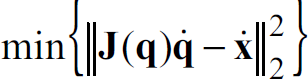
To realize the desired end-effector velocity screws computed by a visual servoing control loop, we wish to solve the classical inverse kinematics velocity problem

J (q) \dot{q} = \dot{x}

(1)

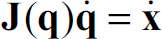
where J(q) is the m × n manipulator Jacobian evaluated for the current robot configuration q, the vector $\dot{q}$ is an n-dimensional vector of joint velocities and $\dot{x}$ is the desired m-dimensional end-effector velocity screw.

When solving this problem for the desired joint velocities $\dot{q}$ , we must however take into account that at any instance, the robot is subject the joint position limit constraints

p_{min} \leq q \leq p_{max}

(2)

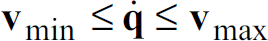
as well as both the joint velocity constraints

v_{min} \leq q \leq v_{max}

(3)

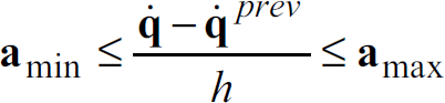
and the joint acceleration constraints

a_{min} \leq \ddot{q} \leq a_{max}

(4)

Here, an arbitrary n-dimensional vector, a is considered less than or equal to another arbitrary vector b of the same dimension if and only if a_i ≤ b_i for i = 1,…, n .

To determine the feasible joint velocities $\dot{q}$ we can express (1) as an optimization problem

min {∥ J (q) \dot{q} - \dot{x} ∥}

(5)

subject to the constraints (2)–(4). When none of the constraints are active, this clearly has the same solution as (1), otherwise we will get the solution, which, according to the selected norm, minimizes the difference between the desired and resulting tool velocity. This formulation has certain advantages over (1), which we will discuss in section 2.3.

In order to efficiently solve this optimization problem, we must express the three constraint types as constraints on the variable $\dot{q}$ , i.e bring the three constraint types on the form

A \leq \dot{q} \leq B

(6)

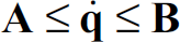
We shall now show, that we can derive appropriate limits A and B directly from the position, velocity and acceleration constraints on the joints.

Obviously, the velocity constraints in (3) are already on this form, and moreover, the joint velocity limits are typically immediately available from the robot specifications. The acceleration and position constraints are, as described in the following, more complicated to handle.

2.1. Acceleration constraints

The joint acceleration limits for a given robot are in general not fixed, but rather functions of the torques, which can be asserted by the individual joint actuators, the loads on the joints and hence also of the robot configuration. The acceleration constraints must hence typically be estimated experimentally or computed using a model of the robot dynamics.

For simplicity in this paper we omit including a complex model of the robot dynamics in our control scheme. We here just propose to use a set of constant worst-case acceleration limits, which ensures that the robot is able to realize at least these joint accelerations in any configuration. If the application does not require the full dynamic potential of the robot, it is often sufficient to make a conservative guess and adjust it based on trial and error. This is the approach we have taken, however if needed the acceleration limits can be estimated more precisely, e.g. by studying the slope of the joint velocity profiles when operating in a high load configuration, or by calculating the dynamical model, as described in (Craig, J.J., 1989).

If the estimated worst-case acceleration limits are given as a_min and a_max as in (4), the constraints imposed by the limited acceleration capabilities of the robot on the joint velocities can be formulated as

a_{min} \leq \frac{\dot{q} - {\dot{q}}^{p r e v}}{h} \leq a_{max}

(7)

where ${\dot{q}}^{p r e v}$ denotes the joint velocity input from the previous control cycle, which now is our current velocity, and h is the cycle time of the control loop. Reorganizing this expression yields

a_{min} h + {\dot{q}}^{p r e v} \leq \dot{q} \leq a_{max} h + {\dot{q}}^{p r e}

(8)

which we will use as our acceleration constraints.

2.2. Position constraints

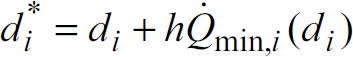
In order to account for joint position limits when computing $\dot{q}$ from (5), these limits must, as expressed by (6), be defined as limits on the joint velocities. Fortunately, this can be achieved by treating each joint individually, hence reducing the complexity of the task.

The cautious choices of velocity and acceleration constraints are to enable the physical robot to follow the specified trajectory very accurately. We may thus make the reasonable basic velocity assumption that if inputs to the low-level controller are given at a rate of h⁻¹ Hz, then the average velocity of the i‘th joint in the time interval [t;t + h], will be between the current velocity ${\dot{q}}_{i}^{p r e v}$ , which we specified at time t – h, and the new velocity ${\dot{q}}_{i}$ , which we at time t specify as the desired velocity at time t + h.

Consider now the i‘th robot joint in an arbitrary position, ${\dot{q}}_{i}^{*}$ . To ensure that any joint motion towards the upper limit, p_max,i, of this joint can be stopped before actually reaching the limit, the velocity of the joint, when arriving at ${\dot{q}}_{i}^{*}$ , must be limited. This upper bound on the allowed joint velocity is defined by the braking capabilities of the robot as well as the distance

d_{i} = p_{max, i} - q_{i}^{*}

(9)

from the current joint position to the upper limit.

In order to compute the maximal allowed joint velocity for the joint at position $q_{i}^{*}$ , we need a worst-case approximation of the distance travelled while braking with the maximal acceleration a_min,i. Using our basic velocity assumption, we can see that the worst-case distance is given by the area under the “stair-case” velocity profile in Fig. 1. We therefore get (remembering that a_min,i is negative) that

h (j + 1) {\dot{q}}_{e n d, i} - h^{2} a_{min, i} \frac{j (j + 1)}{2} = d_{i}

(10)

where by construction the end velocity after j steps are $0 \leq {\dot{q}}_{e n d, i} \leq - h a_{min,}$ .

Fig. 1.

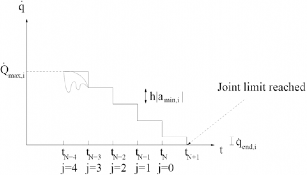
Velocity profile in time domain for joint i. The stair case curve is the worst case curve used to estimate the velocity bounds. Notice, that ${\dot{q}}_{e n d, i}$ is simply the remaining velocity after braking with a_min,i in j steps, and can be expressed as ${\dot{Q}}_{max}$ modulo $h | a_{min, i} |$

We now define the distance d_i as our input computed by (9). We then first wish to compute the integer j. Setting ${\dot{q}}_{e n d, i} = 0$ and solving (10) will give us an upper bound on j, which we shall call j_max

j_{max} = \frac{1}{2} \sqrt{1 - \frac{8 d_{i}}{h^{2} a_{min}, i}} - \frac{1}{2}

(11)

whereas setting ${\dot{q}}_{e n d, i} = - h a_{min, i}$ will give us a lower bound

j_{min} = \frac{1}{2} \sqrt{1 - \frac{8 d_{i}}{h^{2} a_{min}, i}} - \frac{3}{2} = j_{max} - 1

(12)

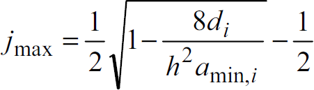
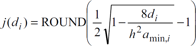
What we are really interested in is the integer between j_min and j_max, which can be defined as a function of d_i as

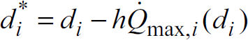
j (d_{i}) = R O U N D (\frac{1}{2} \sqrt{1 - \frac{8 d_{i}}{h^{2} a_{min, i}}} - 1)

(13)

By using (13), we can subsequently solve (10) for the actual value of ${\dot{q}}_{e n d, i}$

{\dot{q}}_{e n d, i} (d_{i}) = \frac{d_{i} + h^{2} a_{min, i} \frac{j (d_{i}) (j (d_{i}) + 1)}{2}}{h (j (d_{i}) + 1)}

(14)

Putting this together we can express the maximal velocity, say ${\dot{Q}}_{max, i}$ , when we are a distance d_i from the limit as

{\dot{Q}}_{max, i} (d_{i}) = {\dot{q}}_{e n d, i} (d_{i}) - j (d_{i}) a_{min, i} h

(15)

Notice that ${\dot{Q}}_{max, i} (d_{i})$ is the maximal velocity allowable at the current position at time t, however we need to find the maximal velocity at time t + h. We therefore need to make a worst-case estimate of the position at time t + h, which, using the basic velocity assumption, will be

d_{i}^{*} = d_{i} - h {\dot{Q}}_{max, i} (d_{i})

(16)

We can now express the limit needed at time t as

{\dot{q}}_{max, i} (d_{i}) = {\dot{Q}}_{max, i} (d_{i}^{*}) = {\dot{Q}}_{max, i} (d_{i} - h {\dot{Q}}_{max, i} (d_{i}))

(17)

Notice from Fig. 1. that ${\dot{q}}_{max, i} (d_{i})$ is only defined when $d_{i} - h {\dot{Q}}_{max, i} (d_{i}) > 0$ , which is automatically assured by the algorithm and the basic velocity assumption.

To determine the maximal allowable joint velocity when moving toward the lower joint limit, we, completely equivalent to the previous derivation, define

d_{i} = q_{i}^{*} - p_{min, i}

(18)

With this definitions, the auxiliary function j(d_i) is found to be

j (d_{i}) = R O U N D (\frac{1}{2} \sqrt{1 + \frac{8 d_{i}}{h^{2} a_{max, i}}} - 1)

(19)

and

{\dot{q}}_{e n d, i} (d_{i}) = \frac{- d_{i} + h^{2} a_{max, i} \frac{j (d_{i}) (j (d_{i}) + 1)}{2}}{h (j (d_{i}) + 1)}

(20)

We can now, using (19) and (20), define our ${\dot{Q}}_{min, i} (d_{i})$ as

{\dot{Q}}_{min, i} (d_{i}) = {\dot{q}}_{e n d, i} (d_{i}) - j (d_{i}) a_{max, i} h

(21)

To complete the derivation, we make the same distance approximate as before

d_{i}^{*} = d_{i} + h {\dot{Q}}_{min, i} (d_{i})

(22)

which can be used to compute the lower limit as

{\dot{q}}_{min, i} (d_{i}) = {\dot{Q}}_{min, i} (d_{i}^{*}) = {\dot{Q}}_{min, i} (d_{i} + h {\dot{Q}}_{min, i} (d_{i}))

(23)

At each control step, we use the above procedure to compute ${\dot{q}}_{min, i} (d_{i})$ and ${\dot{q}}_{max, i} (d_{i})$ , which then can be used as limits in (6). Since the velocities are calculated based on a worst-case scenario, it is important to recalculate them in each step in order to use the entire joint range.

2.3. The Control Objective

As mentioned in section 2, one way to formulate the inverse kinematics problem in velocity space is as the constrained optimization problem in (5) and (6). The norm we wish to minimize is the Euclidean norm, and to simplify things we will look at the square of the norm. Our optimization problem thus becomes

min {{∥ J (q) \dot{q} - \dot{x} ∥}_{2}^{2}}

(24)

subject to

A \leq \dot{q} \leq B

(25)

To avoid having redundant constraints we define the limits A and B as either the position, velocity or acceleration limits according to

\begin{aligned} A_{i} & = max {{\dot{q}}_{m i n, i} (d_{i}), v_{min, i}, a_{min, i} h + {\dot{q}}_{i}^{p r e v}} \\ B_{i} & = min {{\dot{q}}_{m a x, i} (d_{i}), v_{max, i}, a_{max, i} h + {\dot{q}}_{i}^{p r e v}} \end{aligned}

(26)

In Fig. 2, we show A_i as function of d_i. Notice the shift from the constant velocity limit to a distance dependent limit due to the position constraint.

Fig. 2.

The lower limit A_i as a function of the distance d_i from the joint limit

Notice that the constraints in the optimization problem ensure that the physical constraints of the robot are always satisfied, whereas the objective function determines the desired behavior. Notice, furthermore, that we do not require q to be a non-singular configuration, as we shall see in the next section that the matrix J(q)^T J(q) arising in the objective function is only required to be positive semidefinite. This essentially means that we can solve our optimization problem robustly, even in a singular configuration.

When encountering singularities the robots end effector looses one or more degrees of freedom. This however, does not necessarily mean, that it cannot perform the specified motion. Using the optimization scheme, we are able to find proper joint velocities. When a solution does not exist, our approach will simply find the velocity providing the best track.

Unfortunately it does not mean we cannot be trapped in a singularity. If the hyper-plane spanned by the rows of the Jacobian is exactly perpendicular to the desired tool velocity, then due to the Jacobian linearization all motions of the tool would seem to lead it further away from the target, thus the resulting velocity would be 0 for all joints. This type of situation is however very rare, as it requires both that the robot is in a singular configuration, and that the desired tool velocity in the m-dimensional Cartesian space is exactly perpendicular to it. To handle this problem, we would need a higher order approximation than given in (1).

3. Implementation Details

By noticing that the control objective (24) is equivalent to

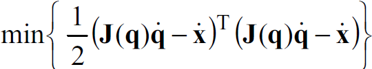
min {\frac{1}{2} (J (q) \dot{q} - \dot{x})^{T} (J (q) \dot{q} - \dot{x})}

(27)

which again is equivalent to

min {\frac{1}{2} {\dot{q}}^{T} J (q)^{T} J (q) \dot{q} - {\dot{x}}^{T} J (q) \dot{q}}

(28)

where the constant term $\frac{1}{2} {\dot{x}}^{T} \dot{x}$ has been removed from the objective function, we can bring our optimization problem on the form of a general quadratic optimization problem in $\dot{q}$ :

min {\frac{1}{2} {\dot{q}}^{T} C \dot{q} - b^{T} \dot{q}}

(29)

subject to

A \leq \dot{q} \leq B

(30)

where, C = J(q)^TJ(q) is a positive semidefinite n × n matrix and $b = {\dot{x}}^{T} J (q)$ .

Notice that even if the configuration q is singular, C is still positive semidefinite, hence a feasible algorithm will still produce a suitable solution such that the computed $\dot{q}$ minimizes the residual error $∥ J (q) \dot{q} - \dot{x} ∥$ .

Several solution methods for such constrained quadratic optimization problems have been developed (Nocedal, J. & Wright, S.J., 1999). Here, we suggest using an approach based on the PATH algorithm developed by Dirkse and Ferris (Dirkse, S.P. & Ferris M.C., 1995). The PATH solver is a stabilized Newton method for solving mixed complementary problems and the algorithm has been shown to be globally convergent. Furthermore, as the algorithm converges super-linearly solutions can be obtained in real-time. To employ this software package, the original problem (28) must however be transformed into a complementary problem.

To perform this conversion, we start by rewriting the n constraints in (25) with upper and lower limits into 2n constraints with only a single limit each. Using the n × n identity matrix I_n we can express these new constraints as

G (\dot{q}) = D \dot{q} + L \geq 0

(31)

where

D = [\begin{matrix} - I_{n} \\ I_{n} \end{matrix}]

(32)

and

L = [\begin{matrix} B \\ - A \end{matrix}]

(33)

We can now use the Karush-Kuhn-Tucker (KKT) conditions (Chong, E.K.P & Zak, S.H., 2001) to obtain a set of equations that are both necessary and sufficient for the solution to the optimization problem. For this we need the gradient of the objective function (29), which is $C \dot{q} - b$ , and the gradient of the constraints, which is simply D. The KKT conditions are then

\begin{aligned} C \dot{q} - b - D^{T} μ & = 0 \\ μ & \geq 0 \\ (D \dot{q} + L)^{T} μ & = 0 \end{aligned}

(34)

where μ represents the 2n constraint multipliers.

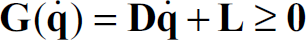
This system can be recognized as a mixed linear complementarity problem, which we can express in matrix form as

[\begin{matrix} C & - D \\ D & 0 \end{matrix}] [\begin{matrix} \dot{q} \\ μ \end{matrix}] + [\begin{matrix} 0 \\ G (\dot{q}) \end{matrix}]

(35)

subject to

G {\dot{q}}^{T} μ = 0, G (\dot{q}) \geq 0, μ \geq 0

(36)

The original control objective is now transformed into a problem, which can be solved for $\dot{q}$ using the PATH software package.

3.1. Performance Considerations

In order to use the proposed control system for real-time visual servoing, it is important that the optimization problem can be solved in sufficiently short time to achieve a reasonable sampling rate.

To ensure that the proposed solution mechanism is suitable, its performance has been evaluated and compared to the widely used active set method (Nocedal, J. & Wright, S.J., 1999), which is generally considered the most effective method for small to medium scale problems.

The two solution strategies have been implemented in a simulation framework and used to simulate numerous control tasks for a seven degrees of freedom Mitsubishi PA10 robot. These experiments have shown that the optimization problem can be solved in less than 1ms on a standard 3.0GHz Pentium IV workstation running Linux and hence that the proposed control algorithm is eminent for visual servoing applications, which require real-time inverse kinematic control of the robot.

Furthermore, the simulations revealed different properties of the two algorithms. In simple tasks, where constraints are only rarely active, the active set method is about twice as fast as the PATH algorithm. However, when increasing the complexity of the tasks and number of constraints needed to be active, the performance of the active set method dropped significantly. The PATH algorithm, on the other hand, proved to be more independent of the input problem, and even though it turned out to be slower on the average, its performance was more constant and provided the fastest worst-case solving time. We thus found it to be the most suitable one for robot control applications.

4. Experimental Evaluation

To evaluate the proposed control system, we have conducted several experiments both in simulation and in real world. The experiments are designed to test various properties of the system as well as to compare our approach to existing techniques. First, to perform the simulated experimental comparison, we have implemented our QP control system as well as a traditional inverse Jacobian method and a selection of the techniques discussed in section 1, into our visual servoing simulator called the VirtualWorkcell (Paulin, M., 2004b). The VirtualWorkcell is a simulation framework, which, contrary to most other robot simulators, is designed for simulation of vision systems and associated robot control methods. It hence not only supports modeling of robot kinematics and visualization of the workcell, but, more importantly, also modeling of real cameras from a set of calibrational parameters as well as methods for rendering camera images offline.

In the simulation system, we have defined the workcell shown in Fig. 3. This workcell consists of a 7 degrees of freedom Mitsubishi PA10 robot and a small cube. To allow eye-in-hand visual servoing of the robot relative to the cube, a camera is mounted near the end-effector of the robot.

Fig. 3.

The setup used for comparison of the visual servoing techniques. Using the end-effector mounted camera for eye-in-hand visual servoing, the robot can be controlled relative to the cube

In the following experiments, the coordinates of two of the corners of the cube, in the image taken by the end-effector mounted camera, are used to implement image based visual servoing of the robot via the control law

\dot{q} = C (λ (s^{*} - s), J_{v})

(37)

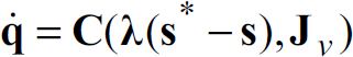
Here, the function C is the control scheme under evaluation. Based on a given proportional gain Λ, a measured distance, s* – s, between the current and the desired image coordinates of the two corners and a stacked version of the standard image Jacobian

J_{v}^{p} = [\begin{matrix} - \frac{f}{z} & 0 & \frac{u}{z} & \frac{u v}{f} & - \frac{f^{2} + u^{2}}{f} & v \\ 0 & - \frac{f}{z} & \frac{v}{z} & \frac{f^{2} + v^{2}}{f} & - \frac{u v}{f} & - u \end{matrix}]

(38)

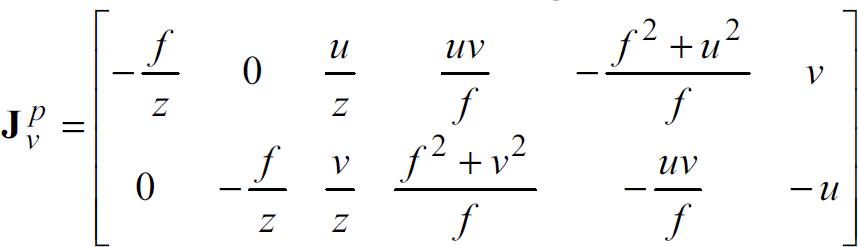
relating camera motions to image plane velocities of a point feature, the controller computes the joint velocities to be realized. In (38), u, v and z are the image coordinates and the depth of the point, respectively, while f is the focal length of the camera.

Besides the traditional inverse Jacobian control method, our QP controller is compared to the previously discussed WLN method (Chan, T.F. & Dubey, R.V., 1995), as well as both the standard GPM technique with singularity avoidance proposed in (Marchand, E.; Chaumette, F. & Rizzo, A., 1996) and the extended iterative GPM method in (Chaumette, F. & Marchand, E. (2001).

These methods are selected as representatives for what seem to be the once most commonly used within the visual servoing community. The use of two point features in (37) constrains four degrees of freedom, leaving three degrees of freedom to the avoidance mechanisms of the various control schemes.

The results presented in the following sections demonstrate the behavior of the selected control systems when joint position, velocity and acceleration limits as well as singularities are encountered during task execution. Furthermore, they verify that our control system, contrary to the other techniques, robustly handles these effects.

4.1. Joint Position Limit Avoidance

To test the joint limit avoidance mechanism of the proposed QP controller, as well as to compare it to the capabilities of the other control schemes, we use the task illustrated in Fig. 4. Using feedback from the end-effector mounted camera, the task is to move the robot from the configuration generating the initial view in Fig. 4(a) to a configuration in which the camera acquires the final view in Fig. 4(b).

Fig. 4.

The image based visual servoing task used to test the joint limits avoidance mechanism of the five control schemes. The straight lines illustrate the ideal trajectories of the two features being used for robot control

The image trajectories of the two features, generated when executing the visual task using the five control schemes, are shown in Fig. 5. As shown in this figure, all control schemes, except the standard inverse Jacobian controller, benefit from their respective joint limit avoidance mechanisms and successfully complete the task, thus generating the desired straight line feature trajectories.

Fig. 5.

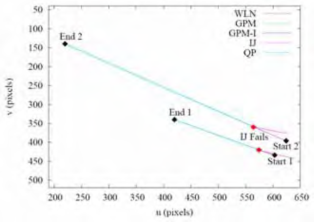
Image trajectories generated by the five control schemes. All but the standard inverse Jacobian controller are able to complete the task. The inverse Jacobian drives the robot into a positional limit which leads to the features moving out of the image

Initially, the inverse Jacobian method is able to execute the task, but since this method has no notion of joint limits and hence does nothing to avoid them, joint four, as shown in Fig. 6, eventually reaches its upper limit. When this event occurs, the robot is no longer able to execute the desired motions and the resulting movements make the image feature move back toward their initial positions and finally out of the image, causing the task to fail.

Fig. 6.

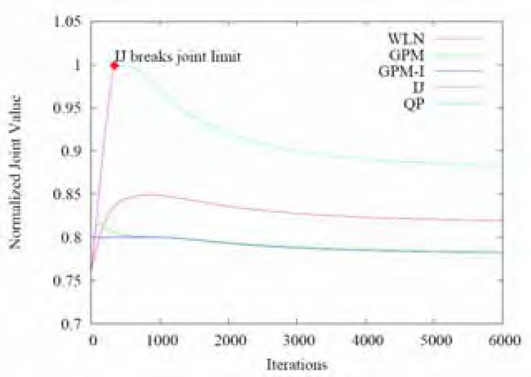
Movement of joint 4 during visual servoing. Notice how the QP method allows the joint to move very close to the limit due to the combined position, velocity and acceleration control

Not until after approximately 1500 iterations does this method allow any motion of the joint and it is hence forced to compensate using the remaining joints. Contrary to the iterative GPM method, the WLN method does not completely block the joint, but simply increases the cost of moving it toward its limit. This makes the joint approach the limit slower than when the robot is controlled using the previous methods.

Also observable from Fig. 6 are the characteristic behaviors of the QP controller as well as of the WLN and iterative GPM methods. Where the QP controller exploits the entire joint range without attempting to break the limit, the iterative GPM method quickly reaches its critical area located at 0.8 in normalized joint coordinates and stops any motion of this joint toward the limit.

It may seem that the choice of 0.8 for the iterative GPM method is somewhat conservative, but one should notice that this choice leaves only ten percent of the joint range in each side, and in the iterative GPM method, the chosen limit may be reached with maximum speed. Moreover, it should be mentioned that the value 0.8 was also used in the original paper about the iterative GPM method.

4.2. Joint Velocity and Acceleration Limits

As expected, all control schemes exploiting the three redundant degrees of freedom to avoid joint limits are able to complete the defined visual task. However, this was done under the assumption that the robot was not constrained by any joint velocity or acceleration limits. In real life, this is not the case, and leaving such constraints out of the control system can severely degrade the performance of the robot.

To allow dynamic effects to be ignored, visual servoing tasks are often executed at very low speeds or under the assumption that the low-level controller and the dynamics of the robot are able to sufficiently smooth the computed motions. Since this approach does not allow exploitation of the full potential of the robot, it is clearly not an acceptable solution in real high-speed applications.

To demonstrate the advantage of explicitly handling joint velocity and acceleration when performing visual servoing control of the robot, we have imposed joint acceleration and velocity limits on the joint velocities computed by the five control schemes when executing the positioning task illustrated in Fig. 4. Instead of the ideal straight line image trajectories in Fig. 5, the degraded trajectories in Fig. 7 are obtained.

Fig. 7.

Image plane trajectories of the two corners of the cube when acceleration and velocity limitations of the real robot are imposed on the computed joint velocities

As expected, these poorer conditions does not improve the performance of the standard inverse Jacobian controller which is still not able to complete the task. More interestingly, it is clear that the limited acceleration and velocity capabilities of the robot have a serious impact on the image trajectories generated by the WLN, GPM and iterative GPM control schemes. As these methods operate under the assumption that any motion can be realized by the robot, the generated image trajectories initially deviate significantly from the desired trajectories. The cause of these deviations is that the error initially is large while the robot is at rest. The motions computed from the discussed control schemes will hence violate acceleration limits and the executed motions will consequently deviate from those computed by the control system. Contrary to the other control schemes, the QP controller is able to generate robot motions which lead to approximately straight line feature trajectories. The reason for this improved performance is clear from Fig. 8. The figure shows the norm of the difference between the desired image plane velocities and those actually achieved when moving the robot, for the first critical part of the visual task, i.e. while the movements are constrained by acceleration limits.

Fig. 8.

Difference between the ideal and achieved image velocities of the visual features

As shown, the velocities realized by the QP controller also initially deviates from the ideal case. However, where the deviations for the other control schemes result in aberrant image trajectories, the deviation, in case of the QP controller, is mainly in the length and not the direction of the velocity vector. One of the key benefits of this new mechanism is that it allows the control system to exploit redundant degrees of freedom to compensate when a joint is constrained by any kind of limit and return joint motions which, in a least squares sense, represent the best possible solution. Consequently, the QP controller reaches a point where the commanded end-effector velocities are actually executable, much faster than the remaining control schemes. This ensures a much better agreement between the desired and the executed motions of the robot. Furthermore, the close integration of acceleration and velocity limits into the control scheme enables the robot to execute a restrained start, which ensures that no limits are violated. This, in turn, results in a smooth motion of the robot, which generate, although slower than in the ideal case, straight line movements of the image features.

4.3. Singularity Handling

The robustness of the proposed QP controller with respect to manipulator singularities is tested using an initial robot configuration in which the end-effector mounted camera is looking down on the cube from straight above. An image based visual servoing task, which attempts to interchange the image positions of the two corners, indicated in Fig. 9, is subsequently executed.

Fig. 9.

View of the cube from the end-effector mounted camera for the initial robot configuration. The task is to make the two indicated corners switch place

As discussed in (Chaumette, F., 1998), this kind of task will result in camera retreat motion, which in turn will result in the robot trying to approach infinity and of course thereby reaching a boundary singularity.

The generated movement of the robot using the QP controller is shown in Fig. 10, while the movements generated by the GPM method is shown in Fig. 11. Except for small variations, the remaining control strategies generate the same robot movements as this approach and exhibit the same behavior when the singularity is encountered.

Fig. 10.

Robot motions generated by the proposed QP-controller. Note, that because the control system is not confined to move the image features along straight lines at all times, the robot is able to complete the task

Fig. 11.

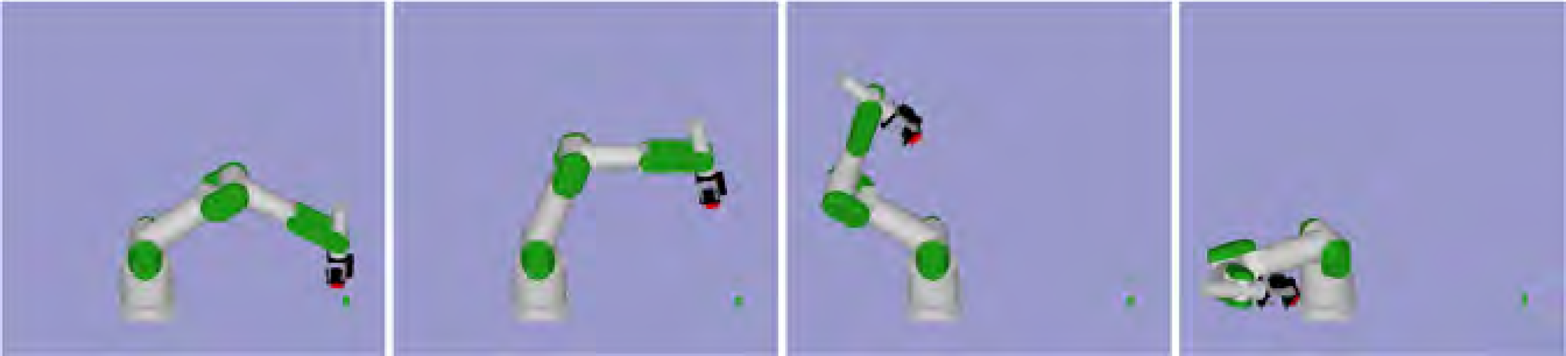
Robot motions generated by the GPM method. Due to camera retreat motions generated by this control law, the system reaches a singularity and the task fails

As illustrated in the figures, the control schemes initially generate similar camera retreat motions in order to make the two image features move toward each other along straight line trajectories. However, when the robot reaches the fully stretched configuration furthest away from the brick, the robot configuration becomes singular. As the QP controller is robust with respect to singularities and, in such situations, is not constrained to move the image features along straight lines, the control scheme simply rotates the camera as this is the optimal motion executable by the robot. Subsequently, the robot is in a configuration where the QP controller is able to generate motions, which realize the optimal path with respect to the visual task, and the image features return to straight line trajectories.

Contrary to the QP controller, the GPM methods, as well as the remaining methods, fail to complete the task when the robot gets in the vicinity of the singular configuration. Although the GPM method does indeed have a singularity avoidance mechanism, this is incorporated as a secondary task executed under the constraint that the primary task is completed. In this case, however, the primary task drives the robot directly into the singularity causing task failure.

To illustrate the uncontrolled behavior of the tested control schemes when the robot is in the vicinity of the singularity, we have removed the joint velocity and acceleration limits on the simulated robot. An example of the joint velocities computed by the five control systems for the first joint is shown in Fig. 12.

Fig. 12.

Normalized velocity of joint 1

In this figure, the joint velocity has been normalized to make the real minimal and maximal joint velocities correspond to -1 and 1, respectively. As the robot approaches the singular configuration, the joint velocities, needed to complete the visual task, for all control systems except the QP controller, become very large. This causes the robot to end up in an aberrant configuration such as the one illustrated in the last picture in Fig. 11. Note from Fig. 12, that the QP controller is able to keep the joint velocities in the allowed range. Due to the explicit handling of velocity and acceleration limits, the QP controller is consequently able to complete the task by compensating for these limits with the remaining joints.

4.4. The RoboCatcher Visual Servoing Application

To verify the proposed control system in a real robotic application, we have implemented the QP control system into our RoboCatcher visual servoing demonstration application. The RoboCatcher setup, shown in Fig 13, is comprised of a Mitsubishi PA10 robot and a stationary camera used to track a small remote controlled car in the playing area. The robot is equipped with a magnetic tool used to catch the car, which is maneuvered by a player. The objective for the player is to get as many points as possible by driving the car into the corner of the playing area, indicated by a flashing diode light, before being caught by the robot.

Fig. 13.

The RoboCatcher eye-to-hand visual servoing application

As we wish to control the robot to catch the car, it is desirable to control the robot to move the TCP in a straight line toward the last detected position of the car. This is achieved by computing the desired end-effector velocity screws using eye-to-hand, position based visual servoing. During servoing, the control system must place the TCP on top of the center of the car and keep the approach vector pointing straight down through the car. As tool roll is not constrained, the task uses 5 of the 7 available degrees of freedom, leaving 2 degrees of freedom redundant.

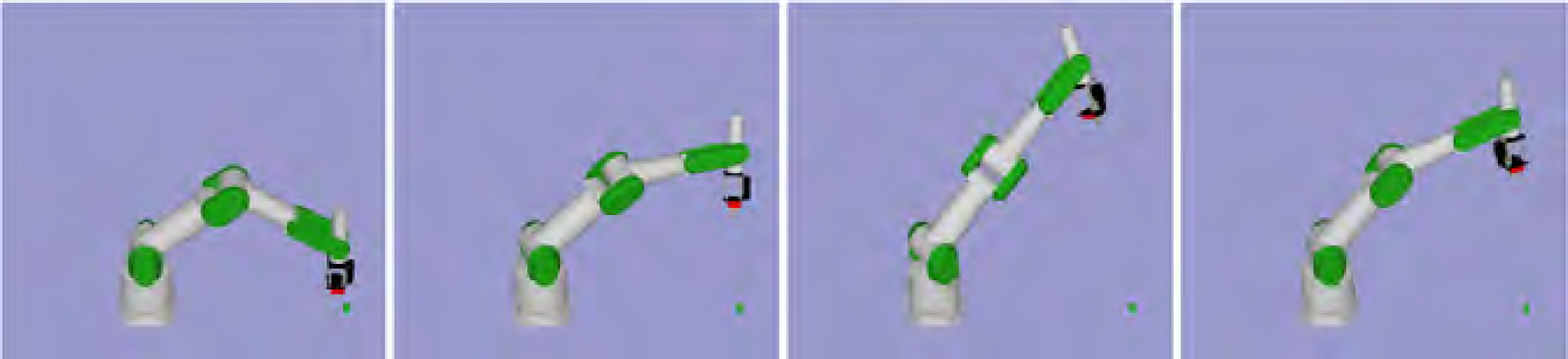
During this experiment, the vision system tracking the car is replaced with a “virtual vision system”, to generate the exact same tasks for all the control schemes. The trajectory imitates a scenario where the car is driving around in a circle with a radius of 0.45m in the playing area in front of the robot. As this circle is centered 0.83m in front of the robot, the car is, on a large segment of its trajectory, out of reach for the robot, which hence encounters a workspace boundary singularity when trying to catch the car. Furthermore, this trajectory brings the car so close to the base of the robot that a joint limit avoidance mechanism is required in order to successfully track the car. To visualize the complete scenario, the configurations of the robot and the car are fed into the VirtualWorkcell. The result of executing the described task using the proposed QP controller is shown in Fig. 14. In the first segment, the car moves close to the robot base. The QP controller avoids reaching the limit of the robot elbow joint by compensating mainly with a rotation of the magnetic tool. When the car start to move away from the base, the robot stretches more and more until the car is out of reach and the workspace boundary singularity has been reached. Because the QP controller is robust with respect to singularities, the robot is able to continue tracking the car, although it cannot reach it. When the car re-enters the workspace of the robot, the QP controller simply blends the path of the TCP into the trajectory of the car.

Fig. 14.

Example of the RoboCatcher visual servoing application using the QP controller. The robot is trying to track the car which moves in a circle in the playing area. The QP control system is robust with respect to singularities which enables the robot to track the car as “good as possible” even if it is out of reach

The “car catching” task has also been executed using the standard inverse Jacobian method, the WLN and versions of the two GPM based methods modified to use position based servoing instead of image based. The result of employing these control techniques are illustrated in Fig. 15. This figure shows the position of the magnetic tool in the plane defined by the playing area. When the task is initiated, both the robot and the car are in their initial positions indicated in the figure. As the car starts moving counter clockwise along the plotted trajectory, the robot moves toward the car and starts tracking it, hence the loop on the paths of the TCP. When the robot reaches the point where the car moves out of reach, every control scheme except the QP controller fails and the task is aborted.

Fig. 15.

Trajectory of the TCP and the car in the plane defined by the playing area

From Fig. 15 it may seem as all control schemes are able to make the robot track the car until the singularity is encountered. However, from inspection of the Cartesian distance between the TCP and the car, plotted in Fig. 16, it is obvious that this is not the case. When the car after approximately 750 iterations is close to the robot base, the standard inverse Jacobian controller reaches a limit of the robot elbow joint and is unable to maintain the desired transformation between the TCP and the car. The result is an increase in the vertical coordinate of the TCP, and hence, as evident from the figure, an increased error. What is more interesting is that the iterative GPM method also fails to accurately track the car in this segments of the reference trajectory. Although this method is able to track the car for 900 iterations by exploiting the secondary task to avoid joint limits, a joint eventually enters its critical area and is stopped. To compensate for this event, some of the remaining joints are commanded to make very rapid movements in the null space of the Jacobian. As these movements cannot immediately be executed by the manipulator due to acceleration and velocity limits, the actual executed movements of the TCP differs from the desired movements computed by the visual servoing control law. The result is an increased tracking error.

Fig. 16.

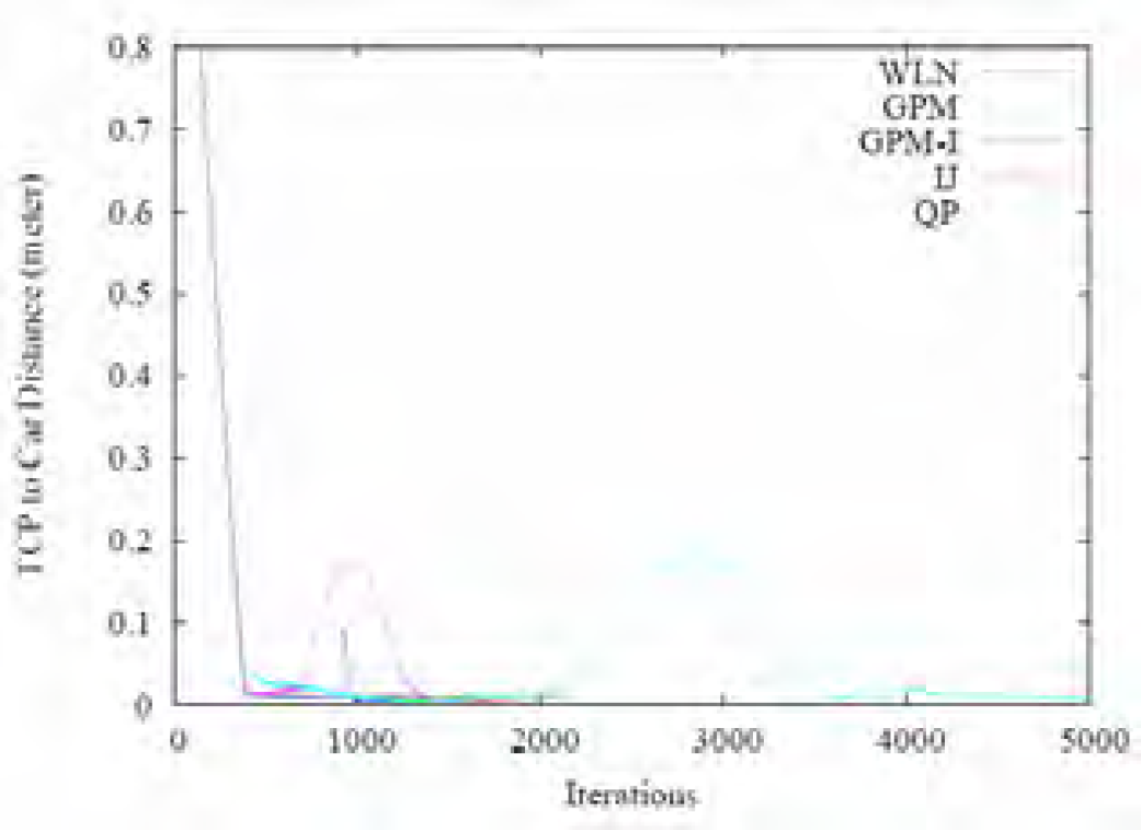
Cartesian distance between the TCP and car during task execution

In agreement with Fig. 15, Fig. 16 illustrates the excellent behavior of the proposed QP controller when the car after 2200 iterations moves out of reach. Until the car move back within reach after 3600 iterations, the robot is, as illustrated in Fig. 14, completely stretched and only rotates the inner-most shoulder joint in an attempt to minimize the distance between the TCP and the car. As the car moves on a circular trajectory, the tracking error increases until the car passes the point on the trajectory furthest away from the robot base. Subsequently, when the car moves back towards the robot, the error decreases until the car is back within reach and again can be accurately tracked by the robot.

5. Conclusion

In this paper we have proposed a novel scheme for controlling robots in visual servoing applications. The presented technique employs quadratic optimization techniques to solve the inverse kinematics problem and explicitly handles both joint position, velocity and acceleration limits by incorporating these as constraints in the optimization process.

Furthermore, as the approach guarantees well-defined joint motions even when the robot is in a singular configuration, the proposed control scheme robustly handles both internal and external singularities.

Contrary to other techniques, which exploit redundant degrees of freedom only to avoid joint position limits, incorporating the dynamic properties of the manipulator directly into the control system enables our method to use redundancy to avoid joint velocity and acceleration limits as well. In turn, this allows faster movements and greater accelerations of the end-effector and hence much better exploitation of the potential of the robot.

The capabilities of the proposed control scheme have been explored in several experiments. In a series of tasks executed in a simulated workcell, we have demonstrated that our control system exhibits superior performance and behavior especially when high end-effector speeds are required. Furthermore, we have evaluated the control system on a real experimental visual servoing platform. These experiments verified that the proposed control system robustly handles singularities and exploits redundancy to avoid joint limits.

Future work aims at extending the proposed control scheme to include linear constraints for collision avoidance. This will enable the robot to avoid obstacles while completing the task specified by the visual control system. In image based visual servoing similar constraints could also be used to guarantee that features never leave the image. Furthermore, we plan to introduce a weight function into the optimization procedure in order to be able to specify the relative importance of motions along the different Cartesian coordinate axes.

References

Chan

T.F.

& Dubey

R.V.

(1995). A Weighted Least-Norm Solution Based Scheme for Avoiding Joint Limits for Redundant Manipulators, IEEE Transactions on Robotics and Automation, Vol 11, pp. 286–292.

Chaumette

(1998). Potential Problems of Stability and Convergence in image-based and position-based visual servoing. The Confluence of Vision and Control, No. 237 in LNCIS, pp. 66–78, Springer Verlag.

Chaumette

& Marchand

(2001). A Redundancy-Based Iterative Approach for Avoiding Joint Limits: Application to Visual Servoing. IEEE Transactions on Robotics and Automation, Vol. 17, pp. 719–730.

Cheng

F.-T.

Chen

T.-H.

& Sun

Y.-Y.

(1992). Efficient algorithm for resolving manipulator redundancy – the compact qp method, Proceedings of the 1992 IEEE International Conference of Robotics and Automation, pp. 508–513, May 1992.

Cheng

F.-T.

Sheu

R.-J.

Chen

T.-H.

& Kung

F.-C.

(1994). The improved compact qp method for resolving manipulator redundancy, Proceedings of the 1994 IEEE/RSJ/GI International Conference on Intelligent Robots and Systems, pp. 1368–1375, 1994

Chong

E.K.P

& Zak

S.H.

(2001). An Introduction to Optimization, Wiley, ISBN: 0-471-39126-3.

Corke

P.I.

& Hutchinson

S.A.

(2000). A New Partitioned Approach to Image-based Visual Servo Control, Proceedings of the 39^th Conference on Decision and Control, pp. 2521–2526, 2000.

Craig

J.J.

(1989). Introduction to Robotics, Mechanics and Control, 2nd Edition. Addision-Wesley, ISBN: 0-201-09528-9

Deng

Janabi-Sharifi & Wilson

W.J.

(2002). Hybrid Strategies for Image Constraints Avoidance in Visual Servoing. Proceedings of the International Conference on Intelligent Robots and Systems, pp. 348–353, Oct. 2002.

10.

Dirkse

S.P.

& Ferris

M.C.

(1995). The PATH Solver: A Non-Monotone Stabilization Scheme for Mixed Complementarity Problems, Optimization Methods and Software, No. 5, pp. 123–156.

11.

Euler

J.A.

Dubey

R.V.

Babcock

S.M.

& Hamel

W.R.

(1989). A comparison of two real-time control schemes for redundant manipulators with bounded joint velocities, Proceedings of IEEE International Conference on Robotics and Automation, pp. 106–112.

12.

Hutchinson

S.A.

Hager

& Corke

P.I.

(1996). A Tutorial on Visual Servo Control. IEEE Transactions on Robotics and Automation, Vol. 12, No. 5, pp. 651–670.

13.

Kwon

Lee

B.H.

& Choi

M.H.

(1999). Resolving kinematic redundancy of a robot using a quadratically constrained optimization technique. Robotica, Vol. 17, pp. 503–511.

14.

Liegeois

(1977). Automatic Supervisory Control of the Configuration and Behavior of Multibody Mechanisms, IEEE Transactions on Systems, Man and Cybernetics, Vol. SMC-7, pp. 686–871.

15.

Malis

Chaumette

& Boudet

(1999). 2 1/2 D Visual Servoing. IEEE Transactions on Robotics and Automation, Vol. 15, No. 2, pp. 238–250.

16.

Mansard

& Chaumette

(2005). A new redundancy formalism for avoidance in visual servoing, Proceedings of IEEE Conference on Intelligent Robots and Systems, IROS'05, pp 1694–1700.

17.

Marchand

Chaumette

& Rizzo

(1996). Using the task function approach to avoid robot joint limits and kinematic singularities in visual servoing. Proceedings of IEEE International Conference in Intelligent Robots and Systems 1996, Vol 3, pp. 1083–1090.

18.

Nocedal

& Wright

S.J.

(1999). Numerical Optimization, Springer Verlag.

19.

Paulin

(2004a). Survey on Visual Servoing in Robotics, Tech. Report. TR2004-8, The Maersk Mc-Kinney Moller Institute for Production Technology, University of Southern Denmark, Mar. 2004.

20.

Paulin

(2004b). The VirtualWorkCell – The Missing Link Between Robot Motion Planning and Visual Servoing, Proceedings of IEEE International Conference on Mechatronics and Robotics, Vol. 2, pp. 326–331.

21.

Samson

Borgne

M.L.

& Espiau

(1991). Robot Control: the Task Function Approach. Oxford Engineering Science Series, Clarendon Press.

22.

Shahamiri

& Jagersand

(2005). Uncalibrated Visual Servoing using a Biased Newton method for On-line Singularity Detection and Avoidance, Proceedings of IEEE Conference on Intelligent Robots and Systems, IROS'05, pp. 2682–2687.

Robust Control for High-Speed Visual Servoing Applications

Abstract

Keywords

1. Introduction

2. Robot Control using Constrained Quadratic Optimization

4. Experimental Evaluation

References