Sage Journals: Discover world-class research

Abstract

Floor storage systems are used in the shoe industry to store fashion products of seasonal collections of low quantity and high variety. Since space is valuable and order picking must be sped up, stacking of shoeboxes should be optimized. The problem is modelled based on shoe features (model, type, colour, and size) and with the goal of forcing similar boxes into locations close to each other in order to improve workers' ability to retrieve orders fast. The model is encoded in Constraint Logic Programming and solved comparing different strategies, also using Large Neighbourhood Search. Simulation experiments are run to evaluate how the stacking model affects picking performance.

Keywords

Fashion shoe industry floor storage systems Storage Location Assignment Constraint Logic Programming Large Neighbourhood Search

1. Introduction

Order picking is generally recognized as the most expensive warehouse operation, because it tends to be very labour- or capital-intensive [1, 2]. Furthermore, it determines the level of service experienced by downstream customers [3].

Studies have shown that if products are stored in convenient locations, they are easier to retrieve when requested by customers, leading to smaller picking times [4]. As underlined in [5], what is meant by “convenience” depends on models of labour and of space. In this research attention is focused on manual floor storage systems in the particular context of the shoe industry. Floor storage systems allow very flexible configurations within a warehouse since no additional structure other than pallets is needed to stack stock keeping units (SKUs). Thus, space can be quickly made available for different SKUs and adapted to their characteristics in terms of size, inventory quantity, and picking frequency; the stocking area can then be easily reconfigured to optimize operations. This is the reason why these simple systems are suitable for industries characterized by seasonal productive campaigns. Furthermore, floor storage systems can be used as a temporary solution in response to volume increases, avoiding other costs while waiting for the construction of more sophisticated structures.

Floor storage systems are often adopted in the shoe industry to manage reorders of collections by retail points during each season. Every shoe model (M) proposed within a seasonal collection can be offered in different material types (T) (leather, tissue, etc.) and colours (C).

Production plants all over the world send cartons containing shoes of identical MTC and sometimes different sizes (S) to satisfy reorders of the main collection during any fashion season. When not all these shoes are required to satisfy client orders during a working period, this produces a certain number of “free pairs”. Free pairs enter the floor storage system, where they are stacked until used to satisfy another retail point demand. Among free pairs, the so-called “fashion products” are proposed only in a given collection and usually with a great variety of MTC combinations. The floor storage system used for the free pairs must manage a great variety of SKUs with very small quantities and hardly predictable arrivals/retrievals during each seasonal collection. Since it is coupled with the other storage systems (the full cartonwarehouse and the classic product warehouse) at the downstream sorting facility, the fashion free pair storage system becomes a potential bottleneck of the whole system. Therefore, any improvement in picking time of fashion free pairs can positively affect the overall response time, even if relatively small quantities are retrieved from the floor storage system during any working period.

Organizing picking operations and optimizing stacking of different shoeboxes within a reasonable number of pallets become important to enhance both fast order retrieval and space-saving. The aim of this paper is therefore to enable fast picking operations through a re-configuration of the floor storage system, according particular attention to the storage location assignment phase. Since real operations show how pickers spend most of their time searching for the required shoeboxes among pallets, the main idea is to speed up the identification process by stacking free pairs based on their model-materials-colour-size (MTCS) features, so that similar shoes are likely to be stored in locations close to each other and pickers can recognize them more easily. To this end, we modelled the problem as a constraints satisfaction problem and encoded it using Constraint Logic Programming. The effectiveness of the proposed optimization model in comparison with common stacking options is proven by simulation: the results show a significant reduction in picking times.

Concerning the optimization methodology, our attention was focused on selecting a solving technique allowing easy encoding and maintainability. To be actually applied in such a dynamic environment as the fashion industry, every mathematical model should be flexible in terms of fast adaptation to changing features of seasonal collections, which reflect on characteristics of the variables and on constraints to be added or modified. Beside flexibility, the particular structure of the problem in the shoe industry should be exploited by ad hoc heuristics and therefore the possibility of customizing techniques also becomes crucial. These considerations have led to the selection of Constraint Logic Programming as the main optimization methodology, which is further enforced by a local search approach to enhance the ability to find very good solutions in reasonable times. Our main goal is to create a conceptual model and a solving tool that can be effectively adopted in real applications: even though other techniques could probably have better computational performance, they are more rigid and the risk of having to start from scratch when passing to the next fashion collection was considered too high.

The paper is organized as follows: a literature review is presented and the best organization for the free pairs picking order system is proposed in section 2. In section 3 the adopted Constraint Programming approach is described; the model for assigning shoeboxes to their locations in the floor storage system is analysed in section 4. In section 5 the implementation of the model is described and computational results are summarized. Simulation experiments, described in section 6, are performed in order to evaluate the proposed model from an operational point of view. Finally, conclusions are proposed in section 7.

2. The manual order picking system: literature review and proposed organization

The three main decisions involved in the order picking process are the storage policy, i.e., how to store the stock-keeping units (SKUs) in the warehouse facilities, the picking policy, concerning which SKUs should be placed on the list of a single picker, and the routing policy, identifying the picking travel path to be followed when retrieving SKUs to fulfil customer orders [2, 6].

Concerning the picking policy, Ackerman [7] identifies three basic picking approaches: strict-order picking, where a picker is responsible for retrieving all the items of a single order per tour; batch picking, where a picker retrieves a set of orders per picking tour; zone picking, where a picker is responsible for retrieving all items stored in a given zone. Two main criteria can be identified for batching [8]: the proximity of pick locations, or time windows. In the latter case, all orders arriving during the same time period are grouped as a batch.

These basic approaches can be combined as described in [9] to form mixed picking strategies. In particular, wave picking can be considered for time-based batching with zone picking, i.e., a picker is responsible for retrieving all SKUs in his zone within a given period (the pick wave). Yu and de Koster [10] developed a queuing network theory model to assess the impact of batching and zoning on the order picking performance of a given system.

In the case of the free pair floor storage system, initial benefits can be achieved by organizing pallets into picking zones corresponding to the different classes of final consumers, i.e., women, men, children, and babies, leading to a family-based storage assignment strategy as described in [11]. This retains the major advantages of zone picking, i.e., the limited space the picker has to traverse to pick an order, the increased familiarity of the picker with a subset of the SKUs, and the reduced order picking time if zones are picked in parallel [3]. In the apparel market the aggregation of SKUs in such families is natural or is induced by speciality catalogues [11].

Since in the analysed shoe firm shipment truck departures are at fixed times within a day, we can fix pick waves so that items retrieved from the floor storage systems and from the carton warehouse can be properly sorted and loaded into trucks.

Petersen and Aase [12] underlined how the capacity of the routing policy to affect time performance in a manual order picking system is significantly lower than for the batching or storage policy. Therefore, we imagine pickers adopting a simple return policy [13], i.e., the picker enters and exits an aisle from the same side, rather than adopting more sophisticated routes such as those recognized in [14] for their Travelling Salesman Problem optimal algorithm, which are rather difficult to be followed by pickers.

Because of the great variety of SKUs and hardly predictable arrivals/retrievals, a picker should be aided in his or her simple route within an aisle of his zone by a storage policy which supports shoebox identification. In the Italian shoe company analysed, a major problem in managing the floor storage system is the time spent by a picker to find the locations where the required shoeboxes are stacked. If shoeboxes were stacked so that a picker could rely on a physical scheme that resembles the aggregation by Model, Type, Colour and Sizes of shoes for a given family, this could be expected to reduce picking time dramatically. This leads to a particular kind of Storage Location Assignment Problem (SLAP), which has been modelled and solved as described in the following sections.

3. The Constraint Programming methodology

The Storage Location Assignment Problem for fashion free pairs can be formalized as a Constraint Satisfaction Problem (CSP), where values representing the MTCS characteristics of shoeboxes to be stored are assigned to available locations (variables), subject to a set of constraints. A cost function can be associated with variable assignments, so that the minimum cost solution can be identified, leading to a Constraint Optimization Problem (COP).

Constraint Programming (CP) is a programming methodology that allows encoding and solving of CSPs and COPs [15]. CP splits problem encoding into two parts: the modelling phase and the solving phase. In the former, the problem is modelled using constraints between variables that need not be linear, unlike in Linear Programming, Integer Linear Programming, or Mixed Integer Programming; non-linear cost functions can also be used. The programmer can then rely on a constraint solver to find solutions. The constraint solver systematically explores the whole solution space, alternating assignment steps with constraint propagation steps. The programmer can improve the performance of this phase by adding heuristics based on the particular structure of the problem.

As underlined in [16], due to their expressive representation constraint-based systems are good for modelling complex problems, including real-life and day-to-day decision-making processes in an enterprise. Compared with techniques such as genetic algorithms, simulated annealing, and tabu-search, they are usually easier to modify and maintain. Moreover, these techniques can be embedded within the search heuristics of a constraint solver, so that advantages of both approaches can be exploited.

Among the various systems for CP, Constraint Logic Programming (CLP) is the most mature constraint programming methodology (the first definition can be traced back to [17]). CLP languages allow a declarative easy encoding, where the focus is on describing properties the desired solution should have, rather than on establishing a procedure to find it.

Free CLP systems such as Gprolog and ECLiPse Prolog are available, as well as commercial systems such as SICStus Prolog and B-Prolog that are easy to install and used in all the platforms, and which allow code portability from one system to another. These characteristics can be suitable especially for small enterprises, traditionally affected by lack of resources, which can access CLP tools at low cost.

CLP has been successfully used in several industrial applications since the 1990s [18], while more recent research fields embrace alert system location [19], computational biology [20], and project-driven manufacturing [16]. Recent surveys on both CLP and its applications can be found in [21].

Thus, CLP is adopted as the main methodology in this paper; however, it is combined with the local search method Large Neighbourhood Search [22] in order to improve its performance.

4. Modelling the storage location assignment problem for fashion free pairs

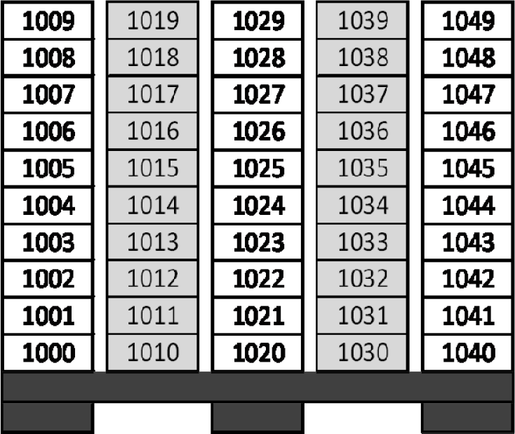
The warehouse is considered as a sequence of floor pallets, organized into aisles. One side of each pallet is associated with a given aisle; the other side belongs to the previous/following aisle (see Figure 1). Given standard sizes of both pallets and shoeboxes, each pallet can contain up to max_col columns of shoeboxes on both sides, stacked up to max_box units (usually max_box ≤ 10 to ensure stack stability), for a maximum of max_col×max_box boxes per pallet side.

Figure 1.

The a-th aisle with 10 pallets in U shape and five boxes/pallet side

Pallets are set in “U shape” and numbered progressively as shown in Figure 1. All available locations (the variables) in our storage system are uniquely identified by a tuple (a, p, c, i) of integers describing the number of the aisle (a), the number of the pallet (p) within a given aisle (p ε [1‥max_pal]), the number of the column c occupied in the pallet (c ε [1‥max_col]), and the slot i (i ε [1‥max_box]) in the analysed column.

The maximum allowed number of pallets per aisle max_pal can be increased during a season to face periods of increasing storage requirements by simple adding pallets at the back front (upper side of Fig. 1). On the other hand, when space-saving becomes crucial in order to devolve space for the successive season collection, max_pal can be reduced.

When warehouse floor size, inventory quantities, and available operators lead to a preference for long aisles, then the model should support different stocking/picking behaviours or a different number of operators for each long front of a given aisle. This can be easily achieved by splitting aisles into their two fronts (left and right sides of aisle axis) and by assigning a different aisle index to each of them in the model.

Each SKU is represented by a shoebox, which is characterized by an integer code ranging from 1000 to 99999.

Thousand digits represent the model of shoes; given the high variety required by fashion products, 99 different models are considered in the current case. The model codes should be assigned consecutively to similar models. Every shoe model can be realized in different materials coded by the hundred digit, thus allowing 10 different combinations (numbered 0-9) per model. Each model-material combination can be proposed to customers in different colours, represented by the decade digit, thus considering 10 alternatives. Finally, shoes are characterized by their size, described in our code by the unit digit. Ten different sizes per shoe model are considered, taking into account the different measures required by men, women, children, and babies. Therefore, an integer code of four to five digits of the type MTCS (Model 1-99, material Type 0-9, Colour 0-9, and Size 0-9) is assigned to each shoebox. If more models/parts/colours/sizes are needed to match with actual cases, the number of related digits can be appropriately increased, moving to greater integers. When a location is assigned to a shoebox, the related variable is set to its MTCS code; otherwise it is set to zero.

4.1 Constraints and cost functions

A set of constraints is imposed so that symmetries of solutions are broken: the goal is to avoid spreading of solutions generated by permutation of the same boxes within a column or the same columns within a pallet. Therefore, columns are filled in a bottom-up way resembling actual stacking of shoeboxes during storage operations. Each pallet is filled from the first to the last column without empty stacks in the middle.

Another set of constraints is related to similarity characteristics of shoeboxes. To force similar shoes to be stacked together, boxes assigned to a column must belong at least to the same shoe model. Thus, all values x_{a,p,c,_} assigned to every location of a given column c in pallet p of aisle a must present the same thousand digits (see Eq. 1, where i and j are any two locations within the same column c). Furthermore, boxes stacked in the same pallet must be characterized by similar models. We define the parameter max_mod as half the length of the range of consecutive models, centred on the first column model. By the constraints in Eq. 2 a number of only 2×max_mod consecutive models can be assigned to a given pallet. For example, if the column 1 model has the code 12 and max_mod is set to 4, then only model codes from 8 to 16 are allowed in that pallet. Max_mod should be selected based on the number of models to be stored in the planning horizon (i.e., fashion models of a seasonal collection) and available columns. When very little space is available in the warehousing system, this constraint should be removed so that model variability within a pallet is enhanced.

int (x_{a, p, c, i} / 1000) = int (x_{a, p, c, j} / 1000) \forall (a, p, c)

(1)

| int (x_{a, p, 1,}_/ 1000) - int (x_{a, p, c,_} / 1000) | \leq {max}_{mod} \forall (a, p, c)

(2)

Finally, the number of non-zero variables (i.e., the locations to be occupied) should be exactly equal to the number of new entering boxes and their values must be chosen from among their integer codes.

When multiple zones are managed together, a family-based allocation should be preserved to enhance pickers' capability of fast retrieval, and constraints linking models of the same family (e.g., woman, man, child, or baby shoes) to a zone (i.e., to a set of aisles) should be added.

To speed up manual retrieval operations, workers should rely on a logical scheme of shoe distribution along aisles, so that similar shoes (i.e., characterized by consecutive integers) are stacked as close together as possible. The cost function C_tot to be minimized is made up of five different contributions, which resemble the proximity requirement of similar shoeboxes, as shown in Equation (3):

C_{t o t} = Σ_{c} (C_{c o l}^{c} + C_{e - c o l}^{c *} + C_{p r o x}^{c *}) + Σ_{p} (C_{p a l}^{p} + C_{e_p a l}^{p *})

(3)

It is desirable to store shoes so that they differ only in size (the unit digit) in the same column, so that workers can easily retrieve them based on client reorders. To force boxes with similar integer codes to enter the same stack, a column cost C^c_col is calculated for every column c with a new entering box, as the sum of the difference between each in-box code and the codes of shoeboxes already stacked, plus the difference of codes between every combination (without repetition) of any two entering boxes assigned to that column. If R is the set of locations within a column already filled with shoeboxes during past replenishments, and V is the set of available locations that are being evaluated for the current solution, then:

\begin{matrix} C_{c o l}^{c} = \sum_{i \in V} \sum_{k \in R} | x_{a, p, c, i} - x_{a, p, c, k} | + \\ Σ_{(i, j) \in V} | x_{a, p, c, i} - x_{a, p, c, j} | \forall (a, p, c) \end{matrix}

(4)

For example, if two boxes with codes 1001 and 1002 are assigned to column s, where a box of code 1000 has already been stacked in a previous replenishment, then the cost of column s will be:

C_{c o l}^{s} = | 1001 - 1000 | + | 1002 - 1000 | + | 1001 - 1002 | = 4

(8)

In order to minimize the number of different shoe codes within a column, the cost contribution is set to zero for a new box with a code already present in the stack, and new boxes with the same code are counted only once for a given column.

To force boxes with the same model, type and colour (MTC) into the same stack without excessive column fragmentation, cost C^c*_{e_col} is introduced to fill a new column (c* in Equation 3). In this way, splitting of boxes differing only by their unit digit (i.e., their size) is discouraged. We set C^c*_{e_col} equal to the column cost Ĉ^c_col in the worst of still-desirable cases, when new boxes are characterized by the same MTC but all different sequential sizes. If codes are sorted in decreasing order, any box code differs from the successive ones for a quantity growing from 1 to its unit value n, as can be seen in Figure 2 for max_box = 10.

Figure 2.

A pallet filled by identical-MTC shoeboxes within a column and by successive colours in stacks

Based on Eq. 4, Ĉ^c_col can be evaluated as:

{\hat{C}}_{c o l}^{c} = \sum_{n = 1}^{({max}_{b o x} - 1)} n (n + 1) / 2

(5)

C^c*_{e_col} should be greater than Ĉ^c_col to discourage a new column occupation, when boxes are characterized by the same MTC. Thus, we set C^c*_{e_col} equal to the nearest integer multiple of 5. In the case shown in Figure 2, where five columns are allowed and 10 boxes are stacked per column, Ĉ^c_col =165 and C^c*_{e_col} =170.

Sometimes, boxes with similar integer codes, can present the same cost C^c_col and could be forced into the same column even if they have different colours (e.g., boxes 1009 and 1011 have two units difference just as boxes 1007 and 1009, but they have different colours, not just different sizes). Thus, a weight equal to C^c*_{e_col} is added to Eq. 4 to distinguish these particular cases, so that filling another column is allowed when enough space is available in the warehouse.

Within a given pallet p, it is desirable to obtain the most similar shoes, so comparisons between all the boxes in that pallet are performed by calculating a pallet cost C^p_pal. This is very similar to the column cost C^c_col, but encompasses all the (max_box×max_col) possible locations, considered as a unique column of max_box×max_col elements. Therefore, the same rules for column cost calculation (see Eq. 4) are applied to the pallet cost component C^p_pal, without adding any weight.

As in the column case, it is desirable to discourage occupation of an excessive number of pallets. In the worst of desirable cases for a new pallet, boxes in each column differ only by size (the unit digit), and columns differ from each other only in their shoe colours (i.e., progressive decade digits are considered). In such a situation, the pallet cost component will be equal to Ĉ^p_pal (see Eq. 6). We introduce a slightly greater empty pallet cost C^p*_{e_pal}, equal to the nearest integer multiple of 10 whenever a new pallet p* is occupied, to avoid splitting of same size and colour boxes among too many pallets.

{\hat{C}}_{p a l}^{p} = \sum_{n = 1}^{(\max_{c o l} \times \max_{b o x} - 1)} n (n + 1) / 2

(6)

Finally, a proximity cost is introduced to force similar shoes to occupy adjacent pallets. This cost component is calculated by the average sum of difference between the model code of any new column c* (see constraints in sect. 4.1) and model codes of non-empty stacks (N̄ in total) occupying the previous and the following pallet, as shown in the following (Eq. 7).

\begin{array}{r} C_{p r o x}^{c *} = \frac{1}{\bar{N}} [\sum_{j = 1}^{\max_{c o l}} | int [\frac{x_{a, p, c *,_}}{1000}] - int [\frac{x_{a, p - 1, j,_}}{1000}] | + \\ \sum_{j = 1}^{\max_{c o l}} | int [\frac{x_{a, p, c *,_}}{1000}] - int [\frac{x_{a, p + 1, j,_}}{1000}] |] \end{array}

(7)

Since cost components have different magnitudes because of the different numbers of pair-wise comparisons involved, weights are introduced in order to counterbalance them.

This problem differs from the classic bin-packing formulation [23], where the aim is maximizing the value of items packed or minimizing wasted space. In our case, instead, space is regarded as a constraint rather than as the objective function, and shoeboxes have no different values. Our goal is to enhance fast picking operations, so pallets can be left empty or only partially filled intentionally, if this is expected to aid pickers in SKU identification. This is also a major difference in comparison with so-called bin-oriented heuristics, in which bins are added and packed one at a time [24]. The analysed problem cannot be considered as variable-size bin-packing, as termed in [25], where bins have different sizes and the goal is to pack items into the set of bins with the smallest total size. Even if during a fashion season stack height (max_box) can be varied based on inventory levels, this constraint is maintained equal for all the pallets within a given picking zone. It cannot even be regarded as an extensible bin-packing problem, as defined in [26], where bins may be extended to hold more than the usual unit capacity. The cost of a bin is 1 if it is not extended, and is equal to its size if it is extended. The goal is to pack a set of items of given sizes into a specified number of bins so as to minimize the total cost. In our case, pallet capacity can be increased as described above; however, the number of pallets to be filled is not an input of the problem, but only a capacity constraint.

5. Solving by Constraint Logic Programming

A program was written in SICStus Prolog to solve the problem, encompassing the three typical steps of the CLP approach: (1) define the domain of each variable; (2) declare problem constraints; (3) search for a good feasible solution or find the optimal one exploring the whole search tree by branch and bound techniques.

Two heuristics are proposed to be used while exploring the search tree, in order to reach good solutions faster than built-in procedures provided by the CLP over finite domains (CLP(FD)) solver of SICStus Prolog [27]. The variable choice heuristic and the value choice heuristic are described in the following sect. 5.1. In sect. 5.2 computational results of the CLP implementation are provided, while in sect. 5.3 a local search approach is added in order to improve performances.

5.1 The search heuristics

The variable-choice heuristic controls the order in which the next variable is selected for assignment. Empty locations in partially occupied columns are selected as the first variables to be assigned, then empty columns in partially occupied pallets are considered, and empty pallets are selected at the end. This selection should force new in-boxes to be stacked near similar already-stored SKUs, whenever possible. To enhance the ability to find good solutions fast, random permutation within the two groups of empty columns is performed.

In the value-choice heuristic, instead, a hierarchical procedure is proposed to identify alternative values to be assigned to a given variable when a branch fail occurs. The following hierarchy of choices is adopted:

The value assigned to the previous selected variable, if different from zero;

A feasible value with same MTC as the last assigned variable, if different from zero, in increasing order;

A feasible value with same MT as the last assigned variable if different from zero, in increasing order;

A feasible value with same M as the last assigned variable if different from zero, in increasing order;

A feasible value with characteristics different from the last assigned one, if different from zero, in increasing order;

If the last assigned value was zero, a feasible positive value should be chosen in increasing order;

Eventually, set the variable to zero, thus leaving the related location empty.

The reference value for the first variable is set to the lowest entering box code. The position of step 7 within the above hierarchy of choice is made dynamic based on the percentage of space available in the floor storage system. When the warehouse has less than 20% of locations already occupied, enough space is available to storage boxes preserving their MTC characteristics, i.e., stacking into the same column boxes differing only by their size. In this case step 7 is shifted soon after step 2 and the selected variable is set to zero immediately after failing step 2. As the number of available locations becomes lower and lower, stacking of boxes with different characteristics in the same or a nearby column becomes more probable. Therefore, step 7 is progressively moved after each following step with every 20% increase of occupied space, becoming the last possible choice if more than 60% of locations are already occupied.

This heuristic, which exploits the features of the analysed problem, was easily encoded in the CLP solver; this would be more difficult in other optimization frameworks (like ILP for instance).

An iterative procedure moving towards lower and lower cost values was implemented in order to find the best feasible solution available when the time-out condition is eventually reached. Its performances are compared to those of the built-in “minimize” procedure, when the number of available locations in the floor storage systems (i.e., the variables) and the number of in-boxes are progressively increased.

5.2 CLP computational results

Experiments were run on a Windows Vista laptop (Intel Core 2 Duo, 2.4 GHz, 3 GB).

Any input configuration can be described by three different parameters: the number of in-boxes to be stored, the size of the floor storage system (i.e., number of locations), and the percentage of locations already occupied. The last two parameters are related to the number of variables to be assigned and therefore to the size of the problem. The former is associated with the number of non-zero variables to be assigned.

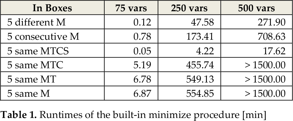
Initially, experiments were performed involving three pallets and five boxes per stack, for a maximum of 75 available locations when the floor storage system were empty, i.e., at the beginning of reorders for a seasonal collection. This relatively small sample allowed testing of all the “minimize” labelling options provided by SictusProlog, which required very similar runtimes (about 7 s). Generally, when entering boxes are more similar (e.g., same M, MT or even MTC) runtimes increase (see Table 1). The variable choice and value choice heuristics do not improve the built-in minimize procedure performance and this is because all the solutions must be generated in order to identify the optimal one.

Table 1.

Runtimes of the built-in minimize procedure [min]

In Boxes	75 vars	250 vars	500 vars
5 different M	0.12	47.58	271.90
5 consecutive M	0.78	173.41	708.63
5 same MTCS	0.05	4.22	17.62
5 same MTC	5.19	455.74	> 1500.00
5 same MT	6.78	549.13	> 1500.00
5 same M	6.87	554.85	> 1500.00

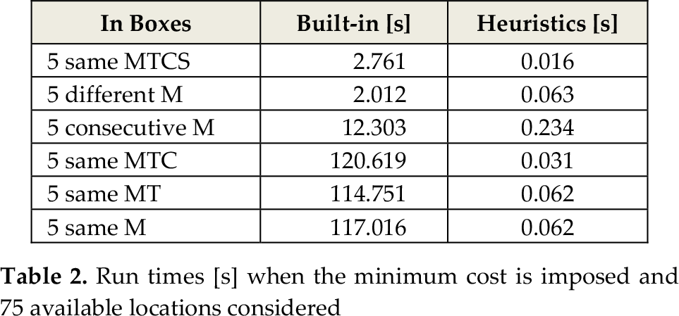
Relative performances of labelling options remain even when a partially filled storage system is adopted (20%, 40%, 60% and 80% of already-filled locations were considered), but runtimes become lower and lower as the number of available locations decreases. The ability of the heuristics to find the best solution faster than the built-in procedures, however, results when fewer than all the solutions are generated, for example when it is required to find the assignment related to a given cost. In Table 2, runtimes of the built-in procedure are compared to those of the proposed heuristics, when the best solution is already known. Heuristics lead to dramatically lower runtimes (from a minimum of 52 times for consecutive M to 3890 times for boxes with same MTC).

Table 2.

Run times [s] when the minimum cost is imposed and 75 available locations considered

In Boxes	Built-in [s]	Heuristics [s]
5 same MTCS	2.761	0.016
5 different M	2.012	0.063
5 consecutive M	12.303	0.234
5 same MTC	120.619	0.031
5 same MT	114.751	0.062
5 same M	117.016	0.062

When the size of the floor storage system is increased in terms of locations to be assigned, and the size of the problem (i.e., the number of variables) consequently grows, runtimes of the minimize approach become unacceptable. With 10 pallets per aisle, several hours are required to reach the optimum, even when only five boxes per column are considered (i.e., 250 variables; see Table 1). If 10 boxes are allowed to be stacked into a column (the extreme situation in real applications), runtimes for some instances exceed one day of computation. Furthermore, increasing the number of entering boxes to be located (i.e., the number of non-zero variables to be assigned) dramatically raises runtimes. For 10 boxes with very different models and 75 available locations, runtime is 4 hours (versus 7.2 seconds for five entering boxes).

By adopting a feasible solution strategy instead of an optimal one, floor storage system size and entering boxes can be increased obtaining good solutions in more reasonable times.

Heuristics prove their force in managing similar entering boxes, which obtained the worst runtimes with the minimize approach (see Table 2). For five same-MT entering boxes we obtained the optimal solution in one iteration in 0.079 s, 0.25 s and 0.749 s for 75, 250, 500 available locations respectively in an empty system, which are dramatically lower times than the related ones in row 5 of Table 1. For five different M boxes, runtime is 0.063 s.

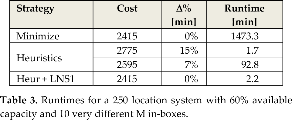
To simulate actual situations in the shoe industry, experiments were run taking into account 10 up to 40 entering boxes and a floor storage system of 10 pallets in one aisle (multiple aisles are managed by a family-based allocation policy and zone picking; therefore, heuristics are supposed to be applied to each family/zone separately). A 60% available storage capacity is considered: for a five-boxes-per-column configuration, 100 filled locations and 150 empty ones are taken into account. With 10 very different M in-boxes, the minimize approach requires about one day of computational time, while the heuristic-based CLP search is able to reach a solution 7% from the optimal one in one hour and a half (see Table 3).

Table 3.

Runtimes for a 250 location system with 60% available capacity and 10 very different M in-boxes.

Strategy	Cost	Δ% [min]	Runtime [min]
Minimize	2415	0%	1473.3
Heuristics	2775	15%	1.7
Heuristics	2595	7%	92.8
Heur + LNS1	2415	0%	2.2

Even if runtime has been drastically reduced, it is still much too long for real applications.

Table 3 highlights how heuristics are able to reach a solution 15% from the optimal one in a very low time (100 s), but further improvements are quite time-consuming. This is the reason why a local search approach was introduced, as explained in the following section.

5.3 Coupling CLP with Large Neighbourhood Search

To further improve the ability to obtain a near-optimal/optimal solution with lower and lower computational times, a local search procedure is added after obtaining a good solution with the above-mentioned heuristics.

In particular a Large Neighbourhood Search (LNS) is adopted [22]. An LNS algorithm is an iterative process that destroys a part of the current solution at each iteration using a chosen neighbourhood definition procedure and re-optimizes it, hoping to find a better solution. The neighbourhood procedure selects a subset of variables, the so-called “free variables” (FV) that should be reassigned, while maintaining the others unchanged as in the current solution. The constraint structure of the model is preserved in order to find only feasible solutions, and this makes LNS particularly suitable to be coupled with Constraint Programming. Moreover, any local search technique is a particular case of LNS, where a small number (typically two) of variables can be chosen as free variables at each iteration.

In our case, top positions of the good solution are randomly made variable again and reassigned in order to lower the cost function. In the first strategy (LNS1), two kinds of moves are allowed for a given solution: two boxes on the top of related columns can be switched, or a box can be removed from the top of its column and stacked on the top of another column. Thus, the first empty location of each column and the top location occupied by an entering box are selected to become FV and be reassigned. The number of FV to be managed by an LNS1 run is kept low by randomly extracting from among the selected top locations (2×max_col×max_pal in the worst case), starting with a narrow group of variables and increasing its size if no improved solutions can be found. To this end, LNS1 resembles a standard local search strategy based on hill climbing.

After obtaining a good solution in a relatively small time (total time-out at 100 s), the iterative LNS1 procedure (sect. 5.3) is added with a global time-out of 100 s, in order to make the improvement phase faster. Results are shown in the last row of Table 3: only 132 s are needed on average to reach the optimal solution.

The number of entering boxes was then increased to 20, 30 and 40 with 10 different models, thus introducing a certain degree of similarity (for 40 boxes, two same-MTCS + two same-MT boxes per model), as the actual “free pairs” generation process suggested. The number of runs for the CLP heuristic phase and the maximum number of runs and time-out per run for the LNS1 phase had to be identified by trial and error to find a proper balance.

Since heuristics (H) are more time–consuming because of the greater number of variables, the mixed CLP + LNS1 approach consists of one iterative heuristic-based procedure and two iterative LNS1 procedures in turn, starting from the same initial good solution (every two LNS1 solutions are compared and the worst discharged). Results for a maximum number of 150 LNS1 runs per time are shown in Table 4).

Table 4.

Results for mixed heuristics (H) + LNS1 strategy

In box	Runs H	Time H [s]	Tout LNS1 [s]	Min cost	Best found cost	Mean cost	Std dev	Total time[min]
20	8	27	2	5152	5152	5174	15	2.6
30	5	96	4	8779	8779	8951	156	5.5
40	3	20	5	13,306	14,177	14,869	411	4.3

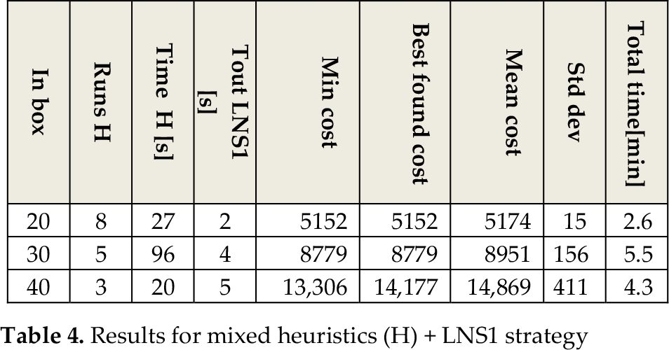
While for 10 and 20 in-box instances performances are very good in terms of both costs and runtimes (see Table 4, last row, and Table 5), the ability of the LNS1 strategy to reach the minimum-cost solution becomes worse and worse as the number of in-boxes is increased up to 40 entering boxes and four boxes per model. Moving only two boxes per time during the LNS phase does not allow very low-cost solutions to be reached, and local minima are encountered. In order to improve performances while maintaining runtimes at reasonably low levels, the LNS2 strategy is introduced.

Table 5.

Results for mixed heuristics (H) + LNS2 strategy

In box	Time H [s]	Runs LNS2	Tout [s]	Min Cost	Best f. cost	Mean cost	Std dev	Δ% min	Total time [min]
30	89	150	4	8779	8779	8847	56	0.8	6.9
40	20	100	8	13,306	13,311	13,463	109	1.2	7.7

In this second strategy, FV identification is based on characteristics of the shoeboxes to be stored: we call maxImod the greatest number of boxes with the same model in the input flow. Thus, we make assignable a random number of locations ranging from 1 to max_Imod of each empty column in the current good solution, i.e., we allow empty columns to be filled in the improved solution. For partially occupied columns, a random number of top locations ranging from 1 to max_Imod are made potentially re-assignable, i.e., we allow some in-boxes to be removed from a column and stacked into another one, if this move improves the solution. To lower the number of FV to be managed by an LNS2 run, however, we randomly extract from among the selected partially occupied columns, increasing the probability of re-assigning as no improved solutions can be found with the current FV cardinality.

FV are then reassigned by using the CLP heuristics strategy, using the iterative backtracking approach. Since LNS2 is itself based on a random extraction of variables, random permutation within the three groups of variables in the variable-choice heuristic (see sect. 5.1) is removed. In this way, we capitalize on the sorting process provided by the CLP heuristics to obtain a good starting solution and leave shifting of boxes to LNS's ability to improve a given configuration faster.

To overcome the problem of local minima typical of a local search approach, LNS2 strategy is empowered with a sort of Monte Carlo method, i.e., the current solution is randomly worsened to allow different search paths to be undertaken.

To keep runtimes as low as possible while decreasing the solution cost, only one iterative LNS2 procedure is performed after the heuristics phase. Results are shown in Table 5.

The percentage difference of the mean cost to minimum cost is drastically lower for the LNS2 strategy than for the LNS1 one (1.17% versus 10.51% for 40 in-boxes); standard deviation of solutions is also reduced. These results confirm how LNS moves should be linked to the number of entering boxes per model to be effective. The best solution found in 10 successive runs equals the minimum cost for 30 in-boxes and approximates it for 40 in-boxes (see Table 5). If a multiprocessor machine is used, several runs can be concurrently launched and therefore the best cost can be detected from among all the solutions found. In this case, there are very good chances of finding the optimal solution in a few minutes.

6. Assessing picking performance by simulation

In order to assess if stacking shoeboxes by the proposed model leads to improved picking time, experiments were performed by using Arena simulation software.

Actual data on arrivals and retrievals of free pairs during a whole seasonal collection were gathered from a well-known Italian shoe company and used in simulation runs.

The “women's” zone was modelled, since female consumers are more sensitive to fashion developments and women's catalogues generally propose the greatest variety of MTC combinations. For the analysed spring collection, 35 different models, with an average of two materials and two colours per model, became free pairs and entered the shop floor system, with 10 boxes per replenishment and five boxes per pick tour on average.

Based on actual data, a single aisle of 10 pallets was sufficient to face fashion free pairs space requirements. The column height was set to five shoeboxes to avoid stack tumble during picking operations, but was increased up to 10 boxes whenever an entering MTCS combination presented more than five units to be stored. When a column is made up of identical shoeboxes, a picker can pull boxes from the top of higher stacks without any fall problem. Therefore, stack height can be increased up to upper bounds of stability, in order to enhance fast identification and space savings.

We imagine storage operations to be performed during idle periods, i.e., when workers are not involved in picking operations (e.g., in later afternoon or early morning). Therefore, the floor storage system is updated with new assignments once a day before pick waves start.

We consider as a basic scenario for comparisons a closest storage policy as termed in [28], or equivalently the “First Fit” heuristic as it is usually called in the bin-packing problem [23]. Every item to be stored is put on the first column on which it fits, starting from partially occupied pallets and opening a new one whenever needed. This choice comes from the evidence stated in [3] that if order pickers could choose the location for storage themselves it would be likely to be the first empty location encountered.

As underlined in [5], one can affect the behaviour of this simple heuristic by choosing how to sort the SKUs on the list. Therefore we tried two different sorting methods: the arriving order in the shop-floor system and the increasing code number. The rationale for the former is to allow replenishments to be split in order to exploit idle periods; for the latter, it is to weakly introduce MTCS characteristics while preserving the First Fit heuristic ease of use. The former heuristic is marked simply as FF and the latter FFmtcs; the proposed storage assignment model is referred to as CLP.

Picking time was split into three main components: travel time, identification time, and handling time. Travel time involves times for entering and exiting the floor storage system and routing among pallets. Identification time is mainly related to the number of boxes a picker should scan in order to recognize the shoe pair to be retrieved, plus other minor contributions for reading the picking list and memorizing box codes. As concerns the handling process, it comprises removing a shoe box from its stack, placing it on the cart and re-stacking boxes dropped on the floor, if necessary. Based on the position of the shoebox to be retrieved within a column, we can differentiate between a slow pick and a fast pick. If the shoebox is on the top, it can be fast removed by the picker, but whenever it occupies middle or bottom locations, extraction time increases, depending on the stack height loading the served location.

The walking speed was set to 110 feet/minute lowering common values for manual picking (see [11, 12, 29]) to adhere to the particular configuration of a floor storage system. Identification and handling times were determined by both time study and predetermined time standards [30].

Results for the analysed women's collection are shown in Figure 3. Picking time is recorded from the moment a picker enters the floor storage system to the moment all free pairs in the picking list have been retrieved and can be moved to the sorting station, where they will be coupled with boxes from the main shelves-based warehouse in order to meet demand. The picking list is completely known when a pick wave starts and no idle times are considered.

Figure 3.

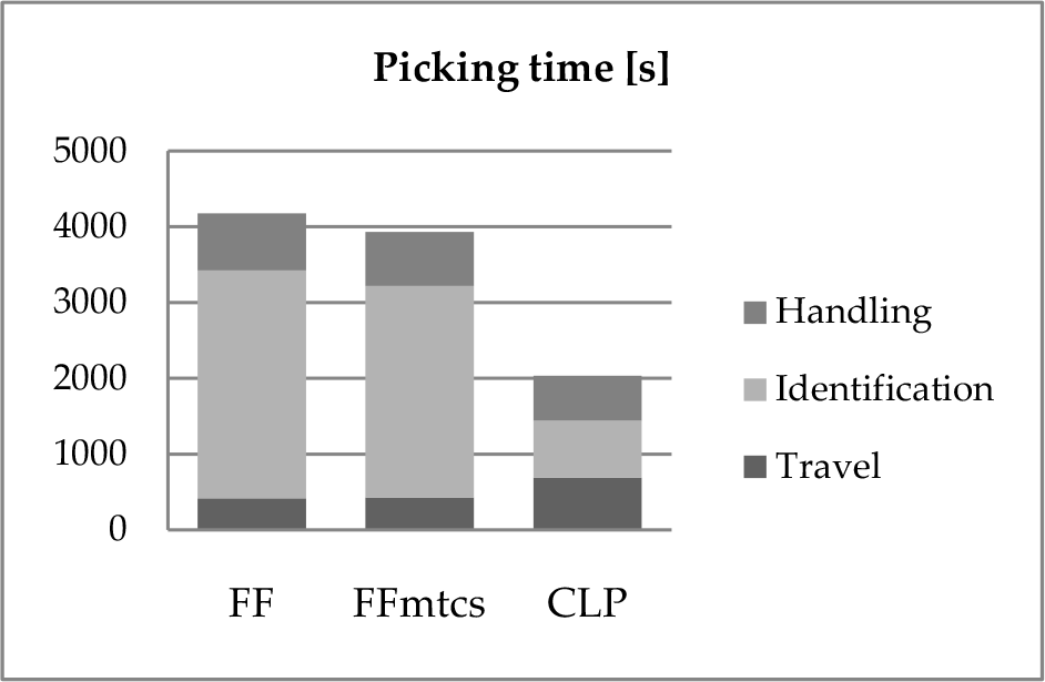
Picking times for First Fit-, FFmtcs- and CLP-based allocations for a whole female collection

Adopting the proposed CLP methodology, 51% total time savings in comparison with FF and 48% in comparison with FFmtcs were achieved across the whole seasonal collection.

As expected, reduction in identification time is the most important contribution: CLP leads to a 75% decrease in comparison with FF and a 73% reduction compared to FFmtcs. This is directly linked to the number of boxes to be scanned. If the CLP storage policy is adopted, a picker can estimate the range of models that are stacked within a pallet by simply reading the code of a single box, due to the constraint in Eq. 2. If none of the boxes to be retrieved can be allocated in the current pallet, he or she can move immediately to the next pallet. With FF and FFmtcs policies, all boxes should be scanned pallet after pallet. Furthermore, with CLP storage a picker can read the code of only the top box in each column to recognize whether it contains the desired model, thanks to the constraint in Eq. 1.

Handling time is also reduced by 21% in comparison with FF and 17% compared to FFmtcs by adopting the CLP policy, since similarity of shoeboxes within a column improves the probability of fast removals.

Travel time, on the other hand, increases by 65% compared with FF and by 61% in comparison with FFmtcs by adopting the CLP policy, because a greater number of pallets is employed to store shoeboxes based on their characteristics, while the First Fit heuristics occupy as few pallets as possible. As can be seen in Figure 3, however, travel time accounts for a minor part of total picking time and therefore it is counterbalanced by improvements gained in the other two time components.

FFmtcs is not able to fully capitalize on MTCS characteristics of shoeboxes to the same extent as the CLP assignment model. Sorting the storage list by MTCS code leads to weak improvements in picking time, but even this highlights how involving MTCS characteristics in assignment models positively affects picking performance.

7. Conclusions

Floor storage systems represent a highly flexible low-cost solution for a temporary inventory or a seasonal business. When a great variety of products in very small quantities should be managed in the short term, the effort of combining space savings and fast picking operations leads to the need for rational allocation of items along aisles and within pallets.

In the shoe industry, where different fashion products are proposed collection after collection, a picker should rely on a logical stacking of shoeboxes, based on their characteristics in terms of model, material, colour and size. In this way, similar products are likely to be stored in positions close to each other and their identification can be faster, even in the absence of sophisticated recognition systems. Simulation experiments show how storing shoeboxes by adopting the proposed shoe features-based allocation model halves total picking time in comparison with common closest-open-location techniques.

Mixing Constraint Programming and Large Neighbourhood Search (thus generalizing either CP or LS) was revealed as a powerful methodology for solving such allocation problems in floor storage systems. Computation times for very good solutions are low enough to allow the proposed methodology to be applied in real warehousing of seasonal low-quantity high-variety products. A case study of a well-known Italian shoe company highlighted how allocations of fashion shoeboxes in the floor storage system are generally performed once or twice per day. Runtimes provided by the CP+LNS solving methodology appear adequate for such a planning period, even when a high number of product classes and aisles should be considered to efficiently manage order picking. Given the complexity of the problem, even with a small number of entering shoeboxes, such timely results could hardly be reached by traditional optimizing approaches.

Furthermore, the declarative nature of CLP allows the programmer to easily describe what properties are required for the desired solution. Requirements can be modified, added or deleted to adapt to a dynamic industrial environment without changing the basic model, only declaring new constraints, which are not limited to being linear. This enables adaptation to and transfer into different industrial realities. Furthermore, search heuristics exploiting the features of the particular problem are easily embedded in the CLP method.

In the analysed decision-making scenario, the flexibility of CLP is invaluable for developing a warehousing tool that can be used collection after collection. Shoe collections differ from one another in seasonal and fashion characteristics, thus affecting stacking requirements. Moreover, different clients' behaviours can impact on picking strategy; storage solutions should therefore be able to speed up operations and offer a quick response to clients, according to the demands of the fashion market. The proposed CLP-based methodology provides the required ability to customize solution properties while still maintaining the basic conceptual model.

References

Tompkins

White

Bozer

Frazelle

Tanchoco

JMA

(2003) Facilities Planning, John Wiley & Sons, New Jersey.

Goetschalckx

McGinnis

(2007) Research on warehouse operation: A comprehensive review. European Journal of Operational Research 177: 1–21.

de Koster

Le-Duc

Roodbergen

(2007) Design and control of warehouse order picking: A literature review. European Journal of Operational Research 182: 481–501.

Sharp

(2001) Warehouse Management. In: Salvendy

, editor. Handbook of Industrial Engineering, John Wiley & Sons, New York 2083–2109.

Bartholdi

III Hackman

(2011) Warehouse & Distribution Science. Release 0.95, Supply Chain & Logistics Institute, Georgia Inst. Tech. Available: http://www2.isye.gatech.edu/~jjb/wh/book/editions/history.html. Accessed 14 May 2013.

Goetschalckx

McGinnis

(2010) Research on warehouse design and performance evaluation: A comprehensive review. European Journal of Operational Research 203: 539–549.

Ackerman

(1990) Practical Handbook of Warehousing. Van Nostrand Reinhold, New York.

Choe

Sharp

(1991) Small parts order picking: design and operation. Georgia Tech Research Corp. Available: http://www.isye.gatech.edu/logisticstutorial/order/article.htm. Accessed November 2010.

Frazelle

Apple

(1994) Warehouse Operations. In: Tompkins

Harmelink

, editors. The Distribution Management Handbook, McGraw-Hill, New York 221–236.

10.

de Koster

RBM

(2009) The impact of order batching and picking area zoning on order picking system performance. European Journal of Operational Research 198: 480–490.

11.

Ruben

Jacobs

(1999) Batch Construction Heuristics and Storage Assignment Strategies for Walk/Ride and Pick Systems. Management Science 45(4): 575–596.

12.

Petersen

Aase

(2004) A comparison of picking, storage, and routing policies in manual order picking. International Journal of Production Economics 92: 11–19.

13.

Hall

(1993) Distance approximations for routing manual pickers in a warehouse. IIE Transactions 25(4): 76–87.

14.

Ratliff

Rosenthal

(1983) Order-Picking in a Rectangular Warehouse: A Solvable Case of the Traveling Salesman Problem. Operations Research 31(3): 507–521.

15.

Rossi

van Beek

Walsh

(2006) Handbook of Constraint Programming, Elsevier Science Inc., New York, USA.

16.

Banaszak

Zaremba

Muszynski

(2009) Constraint programming for project-driven manufacturing. International Journal of Production Economics 120: 463–475.

17.

Jaffar

Lassez

(1987) Constraint Logic Programming. Proceedings of POPL 1987: 111–119.

18.

Jaffar

Maher

(1994) Constraint Logic Programming: A Survey. Journal of Logic Programming 19/20: 503–581.

19.

Avanzini

Rocchesso

Belussi

Dal Palù

Dovier

(2004) Designing an Urban-Scale Auditory Alert System. IEEE Computer 37(9): 55–61.

20.

Dal Palù

Dovier

Fogolari

Pontelli

(2010) CLP-based protein fragment assembly. Theory and Practice of Logic Programming 10: 709–724.

21.

Dovier

Pontelli

(2010) A 25 year perspective on Logic Programming. LNCS 6125, Springer Verlag, Berlin.

22.

Shaw

(1998) Using constraint programming and local search methods to solve vehicle routing problems. Proceedings of CP '98, Springer Verlag, London UK, 417–431.

23.

Johnson

(1974) Fast Algorithms for Bin-Packing. Journal of Computer and System Sciences 8: 272–314.

24.

Fleszar

Charalambous

(2011) Average-weight-controlled bin-oriented heuristics for the one-dimensional bin-packing problem. European Journal of Operational Research 210: 176–184.

25.

Murgolo

(1987) An efficient approximation scheme for variable-sized bin packing. SIAM Journal on Computing 16(1): 149–161.

26.

Coffman

Lueker

(2006) Approximation Algorithms for Extensible Bin Packing, Journal of Scheduling 9: 63–69.

27.

Carlsson

Ottosson

Carlson

(1997) An Open-Ended Finite Domain Constraint Solver. Proc. Programming Languages: Implementations, Logics, and Programs, LNCS 1292, Springer Verlag, 191–206.

28.

Hausman

Schwarz

Graves

(1976) Optimal Storage Assignment in Automatic Warehousing Systems. Management Science 22(6): 629–638.

29.

Chan

FTS

Chan

(2011) Improving the productivity of order picking of a manual-pick and multi-level rack distribution warehouse through the implementation of class-based storage. Expert Systems with Applications 38: 2686–2700.

30.

Matias

(2001) Work measurement: Principles and techniques. In: Salvendy

, editor. Handbook of Industrial Engineering: Technology and Operations Managements, John Wiley & Sons, New York 1410–1462.

Exploiting Fashion Features for Floor Storage Systems in the Shoe Industry

Abstract

Keywords

1. Introduction

2. The manual order picking system: literature review and proposed organization

3. The Constraint Programming methodology

4. Modelling the storage location assignment problem for fashion free pairs

4.1 Constraints and cost functions

5. Solving by Constraint Logic Programming

5.1 The search heuristics

5.2 CLP computational results

5.3 Coupling CLP with Large Neighbourhood Search

6. Assessing picking performance by simulation

7. Conclusions

References