Metal-Insulator Transition from Graphene to Graphane

Abstract

Graphane is obtained by perfectly hydrogenating graphene. There exists an intermediate material, partially hydrogenated graphene (which we call hydrographene), interpolating from pure graphene to pure graphane. Employing a graph theoretical approach to the site-percolation model, we present an intuitive and physical picture revealing a percolation transition from graphene to graphane. It is demonstrated that hydrographene shows a bulk ferromagnetism based on the Lieb theory. We also propose a weighted percolation model in order to take into account the tendency of hydrogenation to cluster.

1. Introduction

Graphene[1, 2] is one of the most interesting material in condensed matter physics. In particular, graphene nanoribbons[3] and graphene nanodisks[4] show remarkable electronic and magnetic properties due to their edge states, and they would be promising candidates for future nanoelectronic devices. Recently graphane has been attracting much attention[5–8]. It is a graphene derivative obtained by perfectly hydrogenating graphene (Fig. 1). On one hand, graphene is a semimetal with each carbon forming an sp² orbital. On the other hand, graphane is an insulator with each carbon forming an sp³ orbital.

Figure 1.

(Color online) (a) Illustration of graphene. There are carbons on a honeycomb lattice. They are grouped in two inequivalent sites A and B. (b) Illustration of graphane. Hydrogens are attached upwardly to A sites, and downwardly to B sites. A honeycomb lattice is distorted.

Carbon atoms in the graphene lattice can bind hydrogens and the reaction with hydrogen is reversible. Accordingly, there exists an intermediate material, partially hydrogenated graphene, which interpolates from pure graphene to pure graphane[7]. Let us call it hydrographene. We expect it to have various intriguing electromagnetic properties.

The hydrogenation of graphene is a complex process that depends on many factors, including the wide isomorphism of cyclohexane. The transient stage of the graphene hydrogenation has been studied at the quantum-chemical level[9–13]. In this paper, however, we propose to explore hydrographene from an unconventional viewpoint, that is, by simulating it on the basis of the percolation model. Percolation theory describes the behavior of connected clusters in a random graph[14]. A comparative examination of the percolation results and the stepwise chemical processes would eventually enrich our understanding of the graphene hydrogenation.

Here, a graph is a network of non-hydrogenated carbons on a honeycomb lattice corresponding to a hydrographene, as illustrated in Fig. 2(a). We next improve this simple percolation model by taking into account the tendency of hydrogenation to cluster. The resultant percolation network seems to capture the basic nature of the experimental observation of hydrographene, as found in Fig. 2(b). We then show that a percolation transition occurs from graphene to graphane at certain hydrogenation density q_c. This is a phase transition since the percolation transition is mapped to a ferromagnet-paramagnet phase transition in a Potts model with q_c corresponding to critical temperature T_c. We also argue that hydrographene is a bulk ferromagnet based on the Lieb theory[16]. The Lieb theory states that the magnetization of the ground states is determined solely by the graph theoretical properties of carbon networks. There are two types of hydrogenation, single-sided (SS) percolation and double-sided (DS) percolation. It is found that SS hydrogenation is more efficient to form large magnetic moment than DS hydrogenation. Though our approach is simple and based on the classical percolation model, it must be a good start point to grasp a gross feature of hydrographene at arbitrary hydrogenation density q.

Figure 2.

(Color online) (a) A typical example of weighted DS percolation network in a honeycomb lattice. Red (blue) circles represent A (B) sites. Solid (open) circles are for dehydrogenated (hydrogenated) sites. (b) Experimental data of hydrographene taken from Balog et al.[7].

2. Model

Graphene is a bipartite system made of carbons at two inequivalent sites (A and B sites) on a honeycomb lattice, as illustrated in Fig. 1(a). It is well described by the Hubbard Hamiltonian,

$H=t\sum _{〈i,j〉}^{}{c}_{\sigma ,i}^{†}{c}_{\sigma ,j}+U\sum _i^{}{c}_{\uparrow ,i}^{†}{c}_{\uparrow ,i}{c}_{\downarrow ,i}^{†}{c}_{\downarrow ,i},$

(1)

where $C_{\sigma ,j}(C_{\sigma ,j}^{†})$ is the annihilation (creation) operator of π-electron with spin σ =↑ ↓ at site i, t is the transfer energy, and Σ_〈i,j〉 denotes the sum over all pairs of nearest-neighboring sites.

Carbon atoms can bind hydrogens. The reaction with hydrogen is reversible, so that the original metallic state and the lattice spacing can be restored by annealing[6]. However, the way of attachment is opposite between the A and B sites in graphane [Fig. 1(b)]. As a matter of convenience, hydrogens are bounded upwardly to A sites and downwardly to B sites.

A hydrographene is manufactured by absorbing a finite density of hydrogens to graphene[7]. Carbons with absorbed hydrogen form an sp³ bond, where no π-electron exists. Hence there is one-to-one correspondence between a hydrographene and a graph made of the honeycomb lattice by removing hydrogenated sites, as illustrated in Fig. 2(a). There exists the Hamiltonian that has one-to-one correspondence to the adjacency matrix of a graph. It is given by the Hubbard Hamiltonian (1) where the lattice points are restricted to the graph in problem: Namely, i runs over all points of the graph and 〈i, j〉 runs over all bonds of the graph. Since the Coulomb interaction in graphene is weak compared to the transfer energy, t >> U, we consider the small interaction limit (U → 0). Namely we analyze the noninteracting model to investigate the zero-energy states,

$H=t\sum _{〈i,j〉}^{}{c}_{\sigma ,i}^{†}{c}_{\sigma ,j}.$

(2)

Although the degeneracy may be resolved for U ≠ 0, the splitting is proportional to U and is small with respective to the band width. This Hamiltonian is block diagonal for σ. Consequently it is enough to investigate the spinless fermion model,

$H=t\sum _{〈i,j〉}^{}{c}_i^{†}{c}_j.$

(3)

The number of the zero-energy states in the model (2) is simply obtained by doubling that in the spinless model (3). As we shall argue later, however, the existence of the Coulomb interaction (U ≠ 0) is important in investigating the magnetization of hydrographene however small it may be.

We can investigate two types of percolation problems in hydrographene. In one case, hydrogenation occurs on both A and B sites, which is DS percolation. In the other case, hydrogenation occurs only on A sites, which is SS percolation. SS hydrogenation can be manufactured by resting graphene on a Silica surface[6].

We analyze a site-percolation problem with the use of the Hamiltonian (3). We first employ the simple percolation model, where hydrogenation is assumed to occur randomly. We then make an improvement of this model. Because adjacent bonds are distorted when one site is hydrogenated, the probability that the next hydrogenation point is contiguous to one of hydrogenated points must become larger owing to a certain energy gain ε, as enhances the tendency of hydrogenation to cluster. We take the effect into account by proposing a weighted percolation model, where a coordination of hydrogenated sites is selected randomly but with the weight given by the Boltzmann factor ^e -βεN _B . Here, N_B counts the total number of the bonds. The clustering is controlled by changing the phenomenological parameter ε. There would arise only one cluster in the limit ε → ∞.

We carry out numerical calculations by setting βε = 1 in this paper. We give a typical carbon network of 30% hydrogenation based on the weighted DS percolation model in Fig. 2(a). The percolation network seems to capture the basic nature of the experimental observation of hydrographene due to Balog et al.[7], as found in Fig. 2(b).

The number of lattice sites with no defects is N_c. We assume N_c is even for simplicity. We define the hydrogenation density by q = M/N_c for DS hydrogenation and q = 2M/N_c for SS hydrogenation, where M is the number of hydrogenated carbons. We choose the positions of hydrogenated carbons by the Monte Carlo method. Physical quantities are determined by taking the statistical average.

3. Isolated carbons

We refer to carbons with no adjacent carbons as isolated carbons, to those with one adjacent carbon as edge carbons, to those with two adjacent carbons as corner carbons, and to those with three adjacent carbons as bulk carbons. We apply a combinatorial theory and estimate the numbers of these different types of carbons by using the fact that each site is occupied with probability q. We also use the quantity p = 1 − q in what follows.

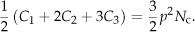
In the case of DS percolation, we calculate the numbers of isolated carbons (C₀), edge carbons (C₁), corner carbons (C₂) and bulk carbons (C₃) as

$\begin{array}{lll}{C}_0=p{q}^3{N}_c,\hfill & C_1=3p^2{q}^2{N}_c,\hfill & C_3=p^4{N}_c.\hfill \end{array}$

(4)

They satisfy the relation

$C_0+C_1+C_2+C_3=p{N}_c.$

(5)

The total bond number is

$\frac{1}{2}(C_1+2C_2+3C_3)=\frac{3}{2}{p}^2{N}_C.$

(6)

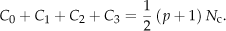
In the case of SS percolation, they are

$\begin{array}{lll}{C}_0=\frac{1}{2}{q}^3{N}_c,\hfill & C_1=\frac{3}{2}p{q}^2{N}_C,\hfill & C_3=\frac{1}{2}(p^3+p)N_C.\hfill \end{array}$

(7)

They satisfy the relation

$C_0+C_1+C_2+C_3=\frac{1}{2}(p+1)N_C.$

(8)

The total bond number is

$\frac{1}{2}(C_1+2C_2+3C_3)=3p{N}_C.$

(9)

We show the numbers of various types of carbons estimated in this way in Fig. 3. In order to verify that the combinatorial theory yields correct results, we have carried out numerical calculations, and found that the results agree completely in the percolation model. There appear some difference in the weighted percolation model. Typically, the number of isolated carbons (C₀) decreases while that of bulk carbons (C₃) increases. As a result, hydrogenation tends to make a cluster.

Figure 3.

(Color online) The numbers of isolated carbons C₀, edge carbons C₁, corner carbons C₂ and bulk carbons C₃ in unit of N_c. Solid (dotted) curves are for the simple (weighted) percolation model. The horizontal axis is the hydrogenation density q. It is seen that C₀ decreases while C₃ increases by the weighted percolation effect.

4. Zero-energy states

We investigate the number of the zero-energy state N₀. It is given by diagonalizing the Hamiltonian. It is equivalently given by the difference between the dimension and the rank of the Hamiltonian,

$N_0=dimH-\text{rank}H,$

(10)

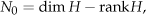
since the number of the zero-energy states is equal to the difference between the dimension of a matrix and the number of the linear dependent element of the matrix. As far as we need only the number of the zero-energy states, it is much easier to calculate (10) than to carry out the direct diagonalization of the Hamiltonian.

The analysis is quite different between DS and SS percolations. We first discuss the DS case. We show the numerical results of the number N₀ in Fig. 4(a) both for the simple and weighted percolation models, where we have adopted the periodic boundary condition to the unit cell with sizes 100.

Figure 4.

(Color online) The number of the zero-energy states determined from eq.(10). Black dots (red open squares) are for the simple (weighted) percolation model. There exists a considerable decrease of the zero-energy states in the weighted percolation model. The unit cell size is 100. The average is taken 1000 times.

Physical interpretations of the zero modes read as follows. In the low density hydrogenation limit (q ≈ 0), all sites are connected, i. e. the cluster number is only one. We can apply the Lieb theorem, which states that the number of the zero-energy states is determined by the difference of the A-site and B-site. It is exactly obtained as

$N_0^{\mathrm{L}}={\sum _{s=0}^M\mid M-2s\mid \left(\begin{array}{c}{N}_C∕2\\ s\end{array}\right)\left(\begin{array}{c}{N}_C∕2\\ M-s\end{array}\right)\left(\begin{array}{c}{N}_C\\ M\end{array}\right)}^{-1}$

(11)

in terms of binomial coefficients. The distribution is symmetric at M = N_c/2. We have shown N₀^L by the choice of N_c = 100 in Fig. 4(a). By taking N_c → ∞, we obtain

$N_0^{\mathrm{L}}=\sqrt{2N_{C}pq∕\pi }.$

(12)

On the other hand, in the high density hydrogenation limit (q ≈ 1), we can apply the dilute gas model. Every sites are isolated or unconnected with each other and give zero-energy states. Then the number of zero is simply given by

$N_0^{\mathrm{D}}=N_C(1-q).$

(13)

We have shown N₀^D by the choice of N_c = 100 in Fig. 4(a).

A simple interpolating formula reads as

$N_0\simeq C_0+\frac{1}{6}{C}_1+\frac{C_2+C_3}{C_0+C_1+C_2+C_3}{N}_0^L,$

(14)

where C₀, C₁, C₂ and C₃ are the numbers of isolated carbons, edge carbons, corner carbons and bulk carbons, respectively. The first and second terms represent the contributions from the isolated and edge carbons, respectively. The third term follows from the Lieb theorem with an appropriate correction. It explains the numerical result reasonably well for the percolation model, as in Fig. 4(a).

On the other hand, there exists a considerable decrease of the zero-energy states in the weighted percolation model. This is because the number of the isolated carbons decreases by the weighted percolation effect.

We now discuss the zero-energy states in SS percolation. The number of the zero-energy states in each cluster is given by

$N_0^{\text{cluster}}=\mid N_B^{\text{cluster}}-N_A^{\text{cluster}}\mid$

in general. Here, N_B^cluster > N_A^cluster since only A sites are hydrogenated. Hence, the total number of the zero-energy states is given by

$N_0=\sum N_0^{\text{cluster}}=N_B-N_A=\frac{1}{2}q{N}_c.$

(15)

This is confirmed perfectly by the numerical result in Fig. 4(b). Thus, the numbers of the zero-energy states are very different between one-sided and DS hydrogenations.

5. Percolation transition

We have calculated numerically the maximum cluster size N^mc as a function of hydrogenation in the system with N_c = 10⁴ based on the simple percolation model and also based on the weighted percolation model, whose results we show in Fig. 5. The ratio N^mc/N_c is approximately equals to the percolation probability P(q). It is by definition the probability for an infinitely large cluster to appear in an infinitely large system. In the present system it may be interpreted as a probability that the right-hand side and the left-hand side of a hydrographene sheet is connected by a cluster.

Figure 5.

(Color online) The maximum cluster size (black dots and red open squares for the simple and weighted percolation models, respectively) and the second maximum cluster size (blue curves) for various hydrogenation density q in unit of N_c. The characteristic feature of a phase transition is clearly observed in both of the models. The unit cell size is 10000.

It is seen in Fig. 5 that the maximum cluster size decreases almost linearly as q increases, and suddenly becomes zero at a critical density q_c. This is a characteristic feature of a phase transition. Indeed, it is a phase transition since the percolation problem is mapped to the zero-state Potts model on Kagomé lattice via the Kasteleyn-Fortuin mapping[15]. The hydrogenation parameter q corresponds to the temperature T of a ferromagnet,

$q=exp(-J∕kT),$

(16)

with J being the exchange stiffness. The percolation probability P(q) is mapped to the magnetization as a function of temperature T. Thus, the percolation transition corresponds to the ferromagnet-paramagnet transition. We anticipate various properties familiar in ferromagnet to be translated into hydrographene via the Kasteleyn-Fortuin mapping.

For DS percolation the critical density is determined as q_c = 0.32, which is consistent with the well-known result[14] on percolation in the honeycomb lattice. We find q_c = 0.55 for SS percolation.

It is to be remarked that the characteristic feature of a phase transition is clearly observed even if the weighted percolation effect is taken into account. This is because the maximum cluster size is rather insensible to isolated carbons.

6. Magnetization

We proceed to analyze the magnetic property of hydrographene. The Lieb theorem[16] plays the key role, which states that the magnetization M of the ground state of the Hubbard model on the connected bipartite lattice at half-filling is determined by the difference between the numbers N_A and N_B of the A and B sites in each cluster,

$M=\frac{1}{2}\mid N_A-N_B\mid ,$

(17)

where the spin direction is arbitrary in general. The theorem is valid for any value of the coupling U provided U ≠ 0. Namely, when U is very small, although the number of zero-energy states is effectively given by the twice of that of the spinless model (3), the magnetization is given by the formula (17). It is important that the magnetization, which is a quantum mechanical property of the ground state, is determined solely by the graph theoretical property of the lattice.

The magnetization of hydrographene is determined by that of the largest cluster: See Fig. 5. This can be understood as follows. The magnetization of each cluster is independent. In the metallic phase, there is only one large cluster with macroscopic order, and all other clusters are very small compared with the largest cluster. The magnetization of a cluster is proportional to its size as in (17). Consequently the main contribution is made by the largest cluster. On the other hand, in the insulator phase, there is no such a cluster with the macroscopic size. Each small cluster has small magnetization, where the direction is independent. Namely, the system shows a paramagnetic behaviour. Small clusters do not contribute to the magnetization. They only contribute to the zero-energy states.

We show the numerically calculated magnetization as a function of q in Fig. 6. It is well approximated by the relation

Figure 6.

(Color online) The magnetization in unit of ħ/2 in the presence (black dots and red open squares for the simple and weighted percolation models, respectively) and absence (blue dots) of ferromagnetic coupling for various hydrogenation density q. The unit cell size is 10000. The average is taken 500 times.

$M(q)=P(q)N_0^{\mathrm{L}},$

(18)

where N₀^L is given by eq.(12) for DS hydrogenation and eq.(15) for SS hydrogenation. The system is ferromagnet for q < q_c, and paramagnet for q > q_c.

The maximum magnetization per site is obtained M = 3 × 10⁻³ at q = 0.21 for DS hydrogenation and M = 0.17 at q = 0.44 for SS hydrogenation. SS hydrogenation is about 500 times more efficient than DS hydrogenation because only A sites are hydrogenated in SS hydrogenation. The magnetization is proportional to the number of the sites. In other words, hydrographene shows the bulk magnetism, which is highly contrasted with the edge magnetism in graphene nanoribbons[3] and nanodisks[4], where magnetization is proportional to the number of carbons along the edge. Bulk magnetism is desirable because edge magnetism disappears in the thermodynamic limit.

A comment is in order. It is intriguing that the magnetization is zero for the perfect SS hydrographene (q = 1), which is in contradiction with the previous result[17] obtained based on a density functional theory study. This is not surprising since the direction of magnetization is arbitrary in each cluster in our noninteracting model, as we have noted. The spin directions of two adjacent clusters may be aligned due to an exchange interaction if it is present, and it is probable that all clusters have the same spin direction. The maximum magnetization per site is obtained around at q = 0.7 for DS hydrogenation: See Fig. 6(a). On the other hand, the magnetization increases linearly as a function of the hydrogenation parameter q for SS hydrogenation: See Fig. 6(b). This reproduces the result[17] for the perfect SS hydrographene (q = 1).

7. Discussions

In summary, we have analyzed hydrographene based on the percolation model. We have shown the existence of a percolation transition in hydrographene. We have proposed a new-type of percolation, SS percolation, which is qualitatively different from the usual percolation on honeycomb lattice.

Carbon network is closely related to the conductance of hydrographene. For q < q_c, there is one large cluster connecting two opposite edges in the sample, and thus the hydrographene would be metallic. On the other hand, the hydrographene would be insulator for q > q_c because there are many small clusters. We may conjecture that a percolation-induced metal-insulator transition would occur at q = q_c. However, the above metal-insulator transition threshold is based on a classical percolation model, which is determined by only the geometrical considerations. Quantum interferences effects due to the randomness of carbon network may lead to localization of the wave function. This Anderson localization results in a lower quantum percolation threshold of metal-insulator transition. To confirm the conjecture, it is necessary to carry out a numerical estimation of conductance, which is beyond the scope of this paper.