Visual Trajectory-Tracking Model-Based Control for Mobile Robots

Abstract

In this paper we present a visual-control algorithm for driving a mobile robot along the reference trajectory. The configuration of the system consists of a two-wheeled differentially driven mobile robot that is observed by an overhead camera, which can be placed at arbitrary, but reasonable, inclination with respect to the ground plane. The controller must be capable of generating appropriate tangential and angular control velocities for the trajectory-tracking problem, based on the information received about the robot position obtained in the image. To be able to track the position of the robot through a sequence of images in real-time, the robot is marked with an artificial marker that can be distinguishably recognized by the image recognition subsystem.

Using the property of differential flatness, a dynamic feedback compensator can be designed for the system, thereby extending the system into a linear form. The presented control algorithm for reference tracking combines a feedforward and a feedback loop, the structure also known as a two DOF control scheme. The feedforward part should drive the system to the vicinity of the reference trajectory and the feedback part should eliminate any errors that occur due to noise and other disturbances etc. The feedforward control can never achieve accurate reference following, but this deficiency can be eliminated with the introduction of the feedback loop. The design of the model predictive control is based on the linear error model. The model predictive control is given in analytical form, so the computational burden is kept at a reasonable level for real-time implementation. The control algorithm requires that a reference trajectory is at least twice differentiable function. A suitable approach to design such a trajectory is by exploiting some useful properties of the Bernstein-Bézier parametric curves. The simulation experiments as well as real system experiments on a robot normally used in the robot soccer small league prove the applicability of the presented control approach.

1. Introduction

Visual servoing (VS) is a technique which uses an image sensor in a feedback loop for motion control of a robot. The field of VS combines robotics, machine vision and control theory. An extensive overview of the VS applications and methodology was given by Corke [1, 2], Chaumette and Hutchinson [3, 4], Kragic and Christensen [5], and Chang [6] etc. Visual servoing can be found in a variety of applications: cooperative movement of mobile soccer robots [7], navigation of autonomous mobile robots [8, 9], docking of autonomous water surface vehicles [10], helicopter and quadrocopter hovering and guidance [11–14], autonomous landing of aeroplanes [15–17], attitude control of satellites [18], grasping and movement of objects [19, 20], and keeping the relative view in a dynamic environment [21] etc.

The VS approaches are normally divided into three main groups [1]: position-based visual servoing (PBVS), image-based visual servoing (IBVS) and hybrid visual servoing. The methods differ in the definition of the control error. In the PBVS case, the control error is defined as the difference between the desired and current pose in the world (Euclidean) space. As opposed to the classical approach of the PBVS, the IBVS (implemented in this paper) defines the control error between the desired and current pose directly in the image coordinate frame (in pixels). The PBVS usually generates better motion, but if the system is not precisely calibrated it may not be able to eliminate the steady-state error. The IBVS can usually achieve an error-free motion, but the generated motion may not be optimum or may sometimes even produce unnecessary or even undesirable motion. The control algorithms that try to combine the useful properties of both approaches are called hybrid VS methods [22]. The VS algorithms may further be divided based on the configuration of the camera and the robot: eye-in-hand and eye-to-hand configuration; and the number of cameras: one camera, two cameras (stereo configuration), multiple cameras (more than two). Some visual servoing approaches take advantage of some special structural properties that can be used implicitly in the design of the control algorithm, e.g., planar surfaces [23]. In this paper we consider an eye-to-hand configuration with one camera. The mobile robot is observed by an overhead camera that is placed at arbitrary inclination with respect to the ground plane. In other words, the arbitrary positioned camera is used to provide information about the position of the mobile robot that moves on a flat surface.

A camera is considered to be an inexpensive and non-invasive sensor, and the information about the environment it provides is extremely rich compared to the other sensors, e.g., laser or ultrasonic distance sensors. This makes the camera an extremely appealing sensor for a broad range of applications. The huge amount of data the images can provide represent a challenge, particularly when it comes to extracting the relevant information for the specific task in real-time. A classical approach to the design of visual servoing consists of image acquisition, image segmentation and classification, high-level reasoning and decision-making, movement planning and, finally, execution of appropriate actions [1]. Although some approaches for visual servoing describe the task on a high (abstract) level [24], the modern approaches consider the action generation directly on the acquired image features to reduce the computational burden. The main idea is that the complex image signal can be described by a relatively small set of image features (like SIFT [25]), and these features are then used in the controller for the calculation of the appropriate actions [8, 18]. However, the classical high-level approach is useful in a process when the system is learning a new task, but when the task is learned, the system should carry it at low level to speed up the execution. In this paper, the machine vision is given a task of measuring the position of the robot in the image frame. To simplify and speed up the segmentation of the robot from the surrounding environment, the robot can be equipped with a marker (special colour or pattern) that can be indistinguishably detected by the image recognition system [7, 13].

The problem of designing a controller for trajectory-tracking (smooth movement along the predefined path) is one of the fundamental problems in robotics. Another fundamental problem in robotics is posture stabilization (movement from point-to-point), but we do not discuss this here. Over the years many different approaches have been developed to tackle the trajectory-tracking problem [26–29]. Some methods for trajectory-tracking are also able to accommodate the path on-line for obstacle avoidance [30, 31]. A good overview of the path planning methods can be found in [32].

The main emphasis of this paper is on the following topics:

The trajectory-tracking task is supposed to be given in the image space, and hence the IBVS is adopted as the control scheme.

The design of the control algorithm takes into account arbitrary inclination of the camera with respect to the ground plane.

The system states are estimated from the delayed measurements using a Kalman filter.

The states of the robot needed in the control law are all estimated in the image frame (no explicit conversion to the world frame is made).

The trajectory-tracking control law is developed in the model predictive framework. The entire control algorithm is designed in the discrete space for optimum performance on a digital computer.

For the path planning, the use of parametric curves under perspective projection is studied.

The overall control algorithm was experimentally tested for robustness.

This paper is structured as follows. Section 2 gives an overview of the system along with all the mathematical equations describing the mobile robot and camera. This is followed by section 3 which presents the design of the controller. The system is linearized with the introduction of a non-linear compensator, which is described in section 3.1. In section 3.2 the model predictive control for trajectory-tracking is presented. Since all the states required by the control algorithm are not directly measurable, a state observer in the form of a Kalman filter is needed, which is presented in section 3.3. In section 4 the approach for designing a trajectory based on Bernstein-Bézier splines is presented. Afterwards, section 5 presents experimental results. Finally in section 6, some conclusions are drawn and ideas for future work are presented.

2. System overview

If not specified differently, we use small bold letters (e.g., x) for column vectors, and big bold letters for matrices (e.g., X). If needed, we use the subscript (·) _w to denote the world coordinate frame, (·) _p for the picture coordinate frame, and (·) _c for the camera coordinate frame. To describe the position and orientation of an object in a plane, we use generalized coordinates q ^T _w = [x y φ] and q ^T _p = [u v θ] with respect to the world and image (picture) frame, respectively. For denoting just a point in a plane we use p ^T _w = [x y 1] and p ^T _p = [u v 1] with respect to the world and image coordinate frame, respectively. Note that we distinguish between bold and regular face symbols, and that we may use the same symbol to denote points in homogeneous and non-homogeneous coordinates interchangeably.

The system consists of a two-wheeled differentially driven mobile robot and a camera that observes the robot from an inclined angle with respect to the ground plane, on which the robot can move freely. Next, we describe the kinematic model of the robot and projective transformation of the camera.

2.1. Mobile robot kinematics

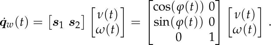
The robot's architecture is shown in Figure 1. The kinematic motion equations of a two-wheeled differentially driven mobile robot are the same as those of a unicycle [32]. The kinematic model has a non-integrable constraint:

Figure 1.

Two-wheeled differentially driven mobile robot.

$$A\left(q_w\right){\dot{q}}_w=\dot{x}\sin \phi -\dot{y}\cos \phi ,$$

(1)

which results from an assumption that the robot cannot slip in a lateral direction. The A ( q _w ) in (1) is the constraint matrix defined over the generalized coordinates q_w. Expressing all the achievable velocities of the mobile robot as a linear combination of the vector fields s_i(q_w) that span the null space of the matrix A ( q _w ) yields the first order kinematic model [32]:

$${\dot{q}}_w\left(t\right)=\left[s_1{s}_2\right]\left[\begin{array}{l}\nu \left(t\right)\\ \omega \left(t\right)\end{array}\right]=\left[\begin{array}{l}\cos \left(\phi \left(t\right)\right)0\\ \sin \left(\phi \left(t\right)\right)0\\ 01\end{array}\right]\left[\begin{array}{l}\nu \left(t\right)\\ \omega \left(t\right)\end{array}\right].$$

(2)

2.2. Camera

The transformation between the world point p ^T _w = [x y z 1] and the corresponding point in the image frame p ^T _p = [u v 1] (in pixels) can be described by a pinhole camera model [33]:

$$\lambda p_p=S\left[Rt\right]p_w,S=\left[\begin{array}{ccc}\alpha & \gamma & u_c\\ 0& \beta & v_c\\ 0& 0& 1\end{array}\right],$$

(3)

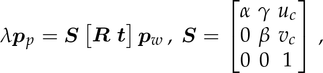
where the λ is a scalar weight, the matrix S holds intrinsic camera parameters, while the matrix R = [r₁ r₂ r₃] ∊ ℝ³ × ℝ³ and vector t ∊ ℝ³ describe the camera orientation and position, respectively. The intrinsic camera parameters contained in the matrix S are: the scaling factors α and β in horizontal and vertical direction, respectively; the optical axis centre (u_c, v_c); and the skew γ. The model is non-linear because of the dependence λ = λ (p_w).

If the world points are confined to a common plane, the relation (3) simplifies. Without loss of generality, we can assume that the plane spans the axis vectors x and y (z = 0):

$$\lambda p_p=S\left[r_1{r}_{2}t\right]p_w=H{p}_w,$$

(4)

where we have taken advantage of the notation by redefining the p ^T _w = [x y 1]. The matrix H ∊ ℝ³ × ℝ³ is known as homography and presents the mapping between the points in the world frame and the corresponding points in the image plane. In a special configuration, when the image frame of the camera is aligned with the world frame, the homography takes a special form:

$$H=\left[\begin{array}{ccc}{s}_u& 0& t_u\\ 0& s_v& t_v\\ 0& 0& 1\end{array}\right],$$

(5)

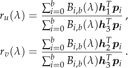
which means that the coordinates of a point in the world plane are just scaled and translated to the image: u = s_ux + t_u and v = s_vx + t_v; where the tuples of values (s_u, t_u) and (s_v, t_v) represent the scaling and translation factor in the horizontal and vertical direction, respectively. Such a canonical configuration can greatly simplify the design of the in plane object tracking, and it is the configuration used in mobile soccer small league [7]. Denoting H^T = [h₁ h₂ h₃], from the equation (4) follows:

$$u=\frac{h_1^T{p}_w}{h_3^T{p}_w}\text{ and }v=\frac{h_2^T{p}_w}{h_3^T{p}_w}.$$

(6)

Note that the denominator in the equations (6) is equal to the factor λ = h ^T ₃ p_w in the equation (4).

The whole system given with the equations (2) and (6) is multi-variable and non-linear. Furthermore, the system (2) is non-holonomic which makes the visual servoing non-trivial since Brockett's theorem (1983) shows that no linear time-invariant controller can control it [2].

3. Control design

The design of the control law is divided into several subsystems. First, it can be shown that the system under consideration, given in the equations (2) and (6), is a differentially flat system with respect to the position of the robot in the image reference frame [27]. Therefore, the system can be linearized by a non-linear dynamic compensator. Based on the obtained linear model, a model predictive control for trajectory-tracking is derived. Since some states needed in the controller are not directly measurable, they must be estimated, and this is achieved with the use of a Kalman filter. The overall control scheme is shown in Figure 2.

Figure 2.

Control scheme. (Operator D denotes the differentiation.)

3.1. Dynamic feedback linearization

How the property of differential flatness can be used in the design of trajectory-tracking and posture stabilization controllers for mobile robots has already been shown in [34]. The control method was later extended to a case where the camera is observing the mobile robot from an arbitrary inclination [26, 27]. Here, we give a brief summary of the approach for dynamic feedback linearization of the system.

A general guideline to obtaining a dynamic feedback compensator is to successively differentiate the system outputs until the system inputs appear in a non-singular way [34]. At some stage, an introduction of integrators on some of the inputs may be necessary to avoid subsequent differentiation of the original inputs.

Let us find the first derivative of the equation (6) with respect to time:

$$\left[\begin{array}{c}\dot{u}\\ \dot{v}\end{array}\right]=\frac{1}{p_w^T\left(h_3{h}_3^T\right)p_w}\left[\begin{array}{c}{p}_w^T\left(h_3{h}_1^T-h_1{h}_3^T\right)\\ p_w^T\left(h_3{h}_2^T-h_2{h}_3^T\right)\end{array}\right]{\left[\begin{array}{ccc}1& 0& 0\\ 0& 1& 0\end{array}\right]}^T\left[\begin{array}{c}\dot{x}\\ \dot{y}\end{array}\right]=F\left[\begin{array}{c}\dot{x}\\ \dot{y}\end{array}\right],$$

(7)

where F ∊ ℝ₂ × ℝ₂, since the matrix F gives the relation between the derivatives of non-homogeneous vectors. Taking into account the equation (2), the relation (7) becomes

$$\left[\begin{array}{c}\dot{u}\\ \dot{v}\end{array}\right]=F\left[\begin{array}{c}\cos \left(\phi \right)\\ \sin \left(\phi \right)\end{array}\right]v.$$

(8)

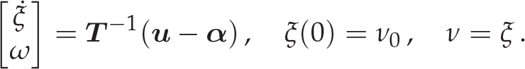
All the inputs have not yet appeared in the equation (8), so we need to continue with the differentiation. However, another differentiation of the equation (8) would differentiate the system input v, so we need to introduce a new state ξ = v before continuing. The second derivative is then:

$$\left[\begin{array}{c}\dot{u}\\ \dot{v}\end{array}\right]=\dot{F}\left[\begin{array}{c}\cos \left(\phi \right)\\ \sin \left(\phi \right)\end{array}\right]\xi +F\left(\left[\begin{array}{c}-\xi \sin \left(\phi \right)\\ \xi \cos \left(\phi \right)\end{array}\right]\dot{\phi }+\left[\begin{array}{c}\cos \left(\phi \right)\\ \sin \left(\phi \right)\end{array}\right]\dot{\xi }\right).$$

(9)

In the equation (9) the other system input (the angular velocity $\omega =\dot{\phi }$ ) appeared, so the process of differentiation can be finished. The equation (9) can be rewritten into a short matrix form:

$$\left[\begin{array}{c}\dot{u}\\ \dot{v}\end{array}\right]=\alpha +T\left[\begin{array}{c}\dot{\xi }\\ \omega \end{array}\right]=\left[\begin{array}{c}{u}_1\\ u_2\end{array}\right]=u.$$

(10)

It can be shown that in a case where the tangential velocity differs from zero v = ξ ≠ 0, and the matrix F is invertible, the matrix T is also invertible, so the dynamic compensator can be expressed from the equation (10) as follows:

$$\left[\begin{array}{c}\dot{\xi }\\ \omega \end{array}\right]=T^{-1}\left(u-\alpha \right),\xi \left(0\right)=v_0,v=\xi .$$

(11)

The elements of the matrix F depend on the world point p_w, but since the world point can be expressed in terms of the image point p_p according to the equation (4), the matrix can be said to depend on the image point: F = F (p_p). Similarly, since the angle φ can be expressed in terms of the values in the image frame:

$$\tan \phi =\frac{\left(h_{21}-v{h}_{31}\right)\dot{u}-\left(h_{11}-u{h}_{31}\right)\dot{v}}{\left(h_{12}-u{h}_{32}\right)\dot{v}-\left(h_{22}-v{h}_{32}\right)\dot{u}},$$

(12)

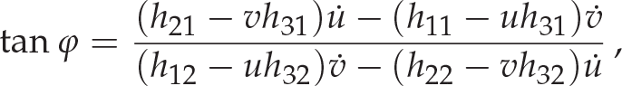
all the terms on the right-hand side of the equation (11) can also be expressed in terms of the values in the image frame: $\alpha =\alpha \left(p_p,{\dot{p}}_p\right)$ and $T=T\left(p_p,{\dot{p}}_p,\xi \right)$ . This is an important observation, because it enables us to estimate all the states, needed in the design of the control law, in the image frame directly.

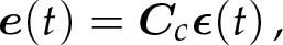
Since the number of differentiations of all the outputs (2 + 2) equals to the order of the original system plus the number of added integrators during the process of differentiation (3 + 1), the overall extended system can be written in the following form:

$${\dot{x}}_i\left(t\right)=A_c{x}_i\left(t\right)+B_c{u}_i\left(t\right),y_i\left(t\right)=C_c{x}_i\left(t\right),$$

(13)

for i ∊ {1, 2}, where $x_1^T=\left[\begin{array}{cc}u& \dot{u}\end{array}\right],x_2^T=\left[\begin{array}{cc}v& \dot{v}\end{array}\right],y_1=\left[u\right]$ and y₂ = [v], and the state-space matrices are:

$$A_c=\left[\begin{array}{cc}0& 1\\ 0& 0\end{array}\right],B_c=\left[\begin{array}{c}0\\ 1\end{array}\right],C_c=\left[\begin{array}{cc}1& 0\end{array}\right].$$

(14)

With respect to the new inputs u and flat outputs p_p, the extended system is not only linear but also without input-output cross-coupling. The system is represented with two uni-variable subsystems, each subsystem consists of two integrators connected in series — the scheme known as chain form.

The feedback part of the controller is designed for each of the subsystems, indexed i = {1, 2} in the equation (13), separately. Since both subsystems in the equation (13) have the same form, we omit the writing of the subscript index i.

We are to develop the controller for the extended system as a sum of the feedforward and feedback actions u = u_F + (–u_B). We assume the reference signal has the same dynamics as the subsystem in the equation (13): ${\dot{x}}_r=A_c{x}_r+B_c{u}_r$ , which in our case means that the reference signal must be at least twice differentiable function. We select the feedforward control signal to be equal to the input signal of the reference model: u_F = u_r. The method of constructing such a reference signal is shown in section 4. Then, the model of the error e = y_r – y has the same form as the subsystem in the equation (13):

$$\dot{є}\left(t\right)=A_cє\left(t\right)+B_c{u}_B\left(t\right),$$

(15)

$$e\left(t\right)=C_cє\left(t\right),$$

(16)

where the state-error vector has been introduced: ∊ = x_r – x.

In the development of the error model predictive controller, the discrete equivalent of the error model (15) is needed. By expanding the step-invariant transformation equations into a Taylor series [35, p. 52], the following discrete error model with the sample time T_s is obtained:

$$є\left(k+1\right)=Aє\left(k\right)+B{u}_B\left(k\right),$$

(17)

$$e\left(k\right)=Cє\left(k\right),$$

(18)

where all the matrices are:

$$\begin{array}{lll}A=\left[\begin{array}{cc}1& T_s\\ 0& 1\end{array}\right],\hfill & B\left[\begin{array}{c}\frac{T_s^2}{2}\\ T_s\end{array}\right],\hfill & C=\left[10\right].\hfill \end{array}$$

(19)

3.2. Error model predictive control

The predictive control can be formulated as an optimization problem where we search for the control signal that minimizes some penalty function over finite prediction horizon h > 0 [28, 31]:

$$\begin{array}{lll}J\left(u_B,k\right)\hfill & =\hfill & {\displaystyle \sum _{i=0}^{h-1}}{\epsilon }^T\left(k,i+1\right)Q\left(i+1\right)\epsilon \left(k,i+1\right)+\hfill \\ \hfill & \hfill & +u_B^T\left(k+1|k\right)R\left(i\right)u_B\left(k+i|k\right),\hfill \end{array}$$

(20)

where we have defined the states' error $∊\left(k,i\right)={є}_r\left(k+i|k\right)-є\left(k+i|k\right);$ and the matrices Q (i + 1) and R (i) are positive-definite for i = 0, 1,…, h − 1.

At the current time step k an estimate of the error based on the model (17) at the future time moment k + h can be obtained provided known current states and inputs until the future time k + h − 1:

$$\begin{array}{lll}\epsilon \left(k+h|k\right)\hfill & =\hfill & {\mathbf{\Lambda }}_h\left(k,0\right)\epsilon \left(k|k\right)+\hfill \\ \hfill & \hfill & +{\displaystyle \sum _{i=1}^{h-1}}{\mathbf{\Lambda }}_h\left(k,i\right)B\left(k+i-1|k\right)u_B\left(k+i-1\right)+\hfill \\ \hfill & \hfill & +B\left(k+h-1|k\right)u_B\left(k+h-1\right),\hfill \end{array}$$

(21)

where ${\Lambda }_h\left(k,i\right)=A\left(k+h-1|k\right)\dots A\left(k+i+1|k\right)A\left(k+i|k\right).$ . All the states over the prediction horizon h can be described with an extended system:

$$\overline{є}\left(k\right)=\overline{A}\left(k\right)є\left(k|k\right)+\overline{B}\left(k\right){\overline{u}}_B\left(k\right),$$

(22)

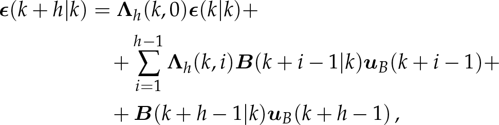
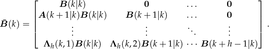
where the predicted states are gathered in the augmented vector $\overline{є}\left(k\right)∊{ℝ}^{n\cdot h}$ :

$${\overline{є}}^T\left(k\right)=\left[{є}^T\left(k+1|k\right){є}^T\left(k+2|k\right)\dots {є}^T\left(k+h|k\right)\right],$$

(23)

and the unknown control inputs in $u_B\left(k\right)∊{ℝ}^{m\cdot h}$ :

$${\overline{u}}_B^T\left(k\right)=\left[u_B^T\left(k|k\right)u_B^T\left(k+1|k\right)\dots u_B^T\left(k+h-1|k\right)\right].$$

(24)

The matrices $\overline{A}∊{ℝ}^{n\cdot h}\times {ℝ}^n$ and $\overline{B}∊{ℝ}^{n\cdot h}\times {ℝ}^{m\cdot h}$ are defined as follows:

$${\overline{A}}^T\left(k\right)=\left[A^T\left(k|k\right)A^T\left(k|k\right)A^T\left(k+1|k\right)\dots {\Lambda }_h^T\left(k,0\right)\right],$$

(25)

$$\overline{B}\left(k\right)=\left[\begin{array}{cccc}B\left(k|k\right)& 0& \cdots & 0\\ A\left(k+1|k\right)B\left(k|k\right)& B\left(k+1|k\right)& \cdots & 0\\ ⋮& ⋮& \ddots & ⋮\\ {\Lambda }_h\left(k,1\right)B\left(k|k\right)& {\Lambda }_h\left(k,2\right)B\left(k+1|k\right)& \cdots & B\left(k+h-1|k\right)\end{array}\right]$$

(26)

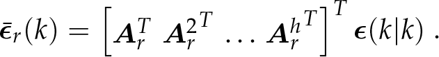
Stacking the reference error states over the prediction horizon h into a vector

$${\overline{є}}_r^T\left(k\right)=\left[{є}_r^T\left(k+1|k\right){є}_r^T\left(k+2|k\right)\dots {є}_r^T\left(k+h|k\right)\right],$$

(27)

the penalty function (20) can be rewritten:

$$J\left({\overline{u}}_B,k\right)={\overline{∊}}^T\left(k\right)\overline{Q}\overline{∊}\left(k\right)+{\overline{u}}_B^T\left(k\right)\overline{R}{\overline{u}}_B\left(k\right),$$

(28)

where

$$\overline{∊}\left(k\right)={\overline{є}}_r\left(k\right)-\overline{є}\left(k\right),$$

(29)

$$\overline{Q}=\underset{i=1}{\overset{h}{{\displaystyle \oplus }}}Q\left(i\right),\overline{R}=\underset{i=0}{\overset{h-1}{{\displaystyle \oplus }}}R\left(i\right).$$

(30)

The operator ⊗ denotes the direct sum. We have the ability to choose the reference error vector ${\overline{є}}_r\left(k\right)$ . One suggestion comes from [28], where the reference error is set to exponentially decrease according to the dynamics defined by the reference model A _r ∊ ℝⁿ × ℝ ⁿ :

$${\overline{є}}_r\left(k\right)={\left[A_r^T{A}_r^{2^T}\cdots A_r^{h^T}\right]}^Tє\left(k|k\right).$$

(31)

Another option is to choose ${\overline{є}}_r\left(k\right)=0$ , which is a special case of the equation (31) when A _r = 0. This option demands from the controller that actual trajectory precisely follows the reference trajectory without filtering the error over the prediction horizon h.

With a search for the minimum of the penalty function $\frac{\partial J\left({\overline{u}}_B,k\right)}{\partial {\overline{u}}_B\left(k\right)}=0$ the optimum inputs to the system are obtained:

$${\overline{u}}_B\left(k\right)={\left({\overline{B}}^T\left(k\right)\overline{Q}\overline{B}\left(k\right)+\overline{\mathrm{R}}\right)}^{-1}{\overline{B}}^T\left(k\right)\overline{Q}\left({\overline{є}}_r\left(k\right)-\overline{A}\left(k\right)є\left(k|k\right)\right).$$

(32)

According to the receding horizon control strategy, at the time instant k only the first m inputs are applied to the system: u _B (k) = [ I 0 … 0]ū _B (k), and at the next time step the whole procedure is repeated again. Because the control law was analytically derived, the need for the time-consuming minimization of the cost function (20) was eliminated, and thus the implementation in real-time systems is possible.

3.3. States estimation

We assume that the image recognition system can provide us with the information about the robot position given in the image frame, however, all the states required for the control are not directly measurable from the image. The unmeasurable states must be estimated, and because we have written the system in a linear form, a Kalman filter can be used. In visual servoing systems, delays are always present, so here we present a design of a Kalman filter that can take delays into account [36].

We assume the outputs of the system (18) are disturbed by a normally distributed white noise with zero mean and covariance matrix N . The states of the system are assumed to be disturbed by a white noise with zero mean and covariance matrix V , filtered by F . Let the delay be equal to d > 0 sample times. In the current moment k, a new measurement of the error e(k_d) is obtained, which was valid at the delayed sample time k_d = k – d. The correction of the posterior $\widehat{є}\left(k_d|k\right)$ with covariance $\widehat{P}\left(k_d|k\right)$ can be made from the estimation ∊(k _d |k − 1) with covariance P (k _d |k − 1):

$$\widehat{є}\left(k_d|k\right)=є\left(k_d|k-1\right)+L\left(k_d|k\right)\left(e\left(k_d\right)-C\left(k_d|k\right)є\left(k_d|k-1\right)\right),$$

(33)

$$\widehat{P}\left(k_d|k\right)=P\left(k_d|k-1\right)-L\left(k_d|k\right)C\left(k_d|k\right)P\left(k_d|k-1\right),$$

(34)

$$L\left(k_d|k\right)=P\left(k_d|k-1\right)C^T\left(k_d|k\right){\left(C\left(k_d|k\right)P\left(k_d|k\right)C\left(k_d|k\right)+N\left(k_d|k\right)\right)}^{-1}.$$

(35)

According to the error model (18), the predictions from the delayed step to the current step can be made:

$$є\left(k|k\right)=\widehat{A}\left(k\right)\widehat{є}\left(k_d|k\right)+\widehat{B}\left(k\right){\widehat{u}}_B\left(k\right),$$

(36)

where we have gathered the last d control signals into augmented vector ${\widehat{u}}_B^T\left(k\right)=\left[u_B^T\left(k_d\right)u_B^T\left(k_d+1\right)\dots u_B^T\left(k-1\right)\right]$ . The matrices $\widehat{A}∊{ℝ}^n\times {ℝ}^n$ and $\widehat{B}∊{ℝ}^n\times {ℝ}^{m\cdot d}$ are defined as follows:

$$\widehat{A}\left(k\right)={\Lambda }_d\left(k,0\right),$$

(37)

$$\widehat{B}\left(k\right)=[{\Lambda }_d\left(k,1\right)B\left(k_d|k\right)\dots {\Lambda }_d\left(k,d-1\right)B\left(k-2|k\right)B\left(k-1|k\right)],$$

(38)

where ${\Lambda }_d\left(k,i\right)=A\left(k-1|k\right)\dots A\left(k_d+i+1|k\right)A\left(k_d+i|k\right)\forall i<d.$ . Before we continue to the next step, we estimate the error in the next delayed step:

$$є\left(k_d+1|k\right)=A\left(k_d|k\right)\widehat{є}\left(k_d|k\right)+B\left(k_d|k\right)u_B\left(k_d\right),$$

(39)

$$P\left(k_d+1|k\right)=A\left(k_d|k\right)\widehat{P}\left(k_d|k\right)A^T\left(k_d|k\right)+\mathrm{FV}\left(k_d|k\right)F^T.$$

(40)

When the Kalman filter is used, it is important that we have accurate estimation of the covariance matrices, otherwise the Kalman filter may return state estimations that are either overconfident or too pessimistic [37].

In multitasking and/or distributed systems it may not be easy to establish sampling time with the constant period which can lead to large errors when we use the equation (36). If the model (18) is known for time-dependent sampling times, the problem can be solved by measuring the time between the samples [13, 36].

4. Trajectory generation

In the development of the control law in section 3.1 we have assumed the reference signal comes from the space of twice differentiable functions. One way of determining the reference trajectory is in the form of a parametric curve (dependent on time) [27, 31, 32]. A convenient way of constructing a reference trajectory is with the use of the Bernstein-Bézier (BB) parametric curves [31]. The BB curves are completely determined with a set of control points, and the number of the control points determine the order of the BB curve. High-order BB curves can be numerically unstable, but it usually suffices to use just low-order curves, since an approximation of an arbitrary curve can be achieved with gluing together more low-order BB curves to obtain a BB spline.

A general D-dimensional BB curve r ^T = [r₁ r₂ … r_D] of order b ∊ 𝒩 in parametric form is defined as follows:

$$r\left(\lambda \right)={\displaystyle \sum _{i=0}^b{B}_{i,b}\left(\lambda \right)p_i,}{B}_{i,b}\left(\lambda \right)=\left(\begin{array}{c}b\\ i\end{array}\right){\lambda }^i{\left(1-\lambda \right)}^{b-i},$$

(41)

where the parameter λ represents the normalized time which takes the real values from the interval [0, 1] and it is related to the relative time t with the linear equation t = λΛ, where Λ is the time it takes to reach from the beginning (λ = 0) to the end (λ = 1) of the curve. The BB curve (41) is of class C_∞ (smooth curve), and it is completely defined by a set of control points {p ^T _i = [p_{1, i} p_2,i … p_D,i]}_i=0,1,…,b that form a Bézier polygon. The BB curve is always bounded by the convex envelope of the Bézier polygon. The derivative of the BB curve with respect to relative time t of order d ≥ 0 is as follows:

$$\frac{{\partial }^{d}r\left(t\right)}{\partial t^d}=\frac{1}{{\mathrm{\Lambda }}^d}\frac{{\partial }^{d}r\left(\lambda \right)}{\partial {\lambda }^d}.$$

(42)

4.1. Bernstein-Bézier curve at end points

The BB curve (41) always begins (λ = 0) at the first control point p₀ and ends (λ = 1) at the last control point p_b; the so-called end point interpolation property. All the other control points in general do not lie on the BB curve. Next, we show how the other control points influence the behaviour of the curve at the end points. At the end points, the following limits can be derived for d ≥ 0, b ≥ d:

$$\underset{\lambda \to 0}{\lim }\frac{{\partial }^{d}r\left(\lambda \right)}{\partial {\lambda }^d}=\left(\begin{array}{c}b\\ d\end{array}\right)d!{\displaystyle \sum _{i=0}^d{\left(-1\right)}^i\left(\begin{array}{c}d\\ i\end{array}\right)}{p}_{d-i},$$

(43)

$$\underset{\lambda \to 1}{\lim }\frac{{\partial }^{d}r\left(\lambda \right)}{\partial {\lambda }^d}=\left(\begin{array}{c}b\\ d\end{array}\right)d!{\displaystyle \sum _{i=0}^d{\left(-1\right)}^i\left(\begin{array}{c}d\\ i\end{array}\right)}{p}_{b-i}.$$

(44)

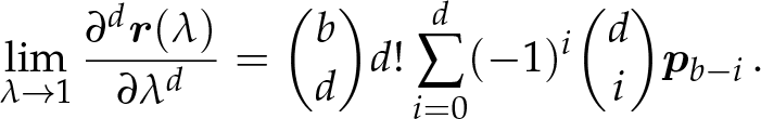
The derivative of order d at the end points is dependent only on the d first or last control points, respectively.

Let us confine ourselves to a two-dimensional space $\left(r^T=\left[\begin{array}{cc}{r}_x& r_y\end{array}\right],p_i^T=\left[\begin{array}{cc}{p}_{x,i}& p_{y,i}\end{array}\right]\right).$ . In this case the orientation of the tangent on the curve is determined by the equation:

$$\phi \left(t\right)=\arctan \frac{{\dot{r}}_y\left(t\right)}{{\dot{r}}_x\left(t\right)}+C\pi ,C∊\mathbb{Z}.$$

(45)

The tangential velocity along the curve is calculated as follows:

$$v\left(t\right)=\sqrt{{\dot{r}}_x^2\left(t\right)+{\dot{r}}_y^2\left(t\right)},$$

(46)

and from the differentiation of the (45), the angular velocity along the curve is obtained:

$$\omega \left(t\right)=\frac{{\dot{r}}_x\left(t\right){\ddot{r}}_y\left(t\right)-{\ddot{r}}_x\left(t\right){\dot{r}}_y\left(t\right)}{{\dot{r}}_x^2\left(t\right)+{\dot{r}}_y^2\left(t\right)}.$$

(47)

We consider only the relations at the starting point of the BB curve (41) (λ = 0), since the relations at the end point can be obtained in the same way. Taking into account the equations (42) and (43), the tangential velocity (46) at the starting point of the BB curve can be expressed in terms of the first two control points:

$$v_0=\underset{t\leftarrow 0}{\lim }v\left(t\right)=\frac{b}{\mathrm{\Lambda }}\sqrt{{\left(p_{x,1}-p_{x,0}\right)}^2+{\left(p_{y,1}-p_{y,0}\right)}^2}.$$

(48)

We assume the tangential velocity never reaches zero v(t) ≠ 0. The orientation (45) at the starting point is then given as:

$${\phi }_0=\underset{t\leftarrow 0}{\lim }\phi \left(t\right)=\arctan \frac{p_{y,1}-p_{y,0}}{p_{x,1}-p_{x,0}}+C\pi ,C∊\mathbb{Z},$$

(49)

and the angular velocity (47) at the starting point as:

$${\omega }_0=\underset{t\leftarrow 0}{\lim }\omega \left(t\right)=\frac{b-1}{\mathrm{\Lambda }}\frac{\left(p_{x,1}-p_{x,0}\right)p_{y,2}-\left(p_{y,1}-p_{y,0}\right)p_{x,2}+p_{x,0}{p}_{y,1}-p_{x,1}{p}_{y,0}}{{\left(p_{x,1}-p_{x,0}\right)}^2+{\left(p_{y,1}-p_{y,0}\right)}^2}.$$

(50)

The relation (50) is the equation of a line that is parallel to the line that passes through the control points p₀ and p₁. When the point p₂ lies on the line passing through the points p₀ and p₁, the angular velocity ω₀ becomes zero. It can be shown that the lines perpendicular to the line that is passing through the points p₀ and p₁ represent the lines of constant tangential acceleration $\dot{v}$ at the starting point as seen from another equation of a line:

$$a_0=\underset{t\leftarrow 0}{\lim }\dot{v}\left(t\right)=\frac{b-2}{{\mathrm{\Lambda }}^2}\frac{\left(p_{x,2}-2p_{x,1}+p_{x,0}\right)\left(p_{x,1}-p_{x,0}\right)+\left(p_{y,2}-2p_{y,1}+p_{y,0}\right)\left(p_{y,1}-p_{y,0}\right)}{{\left(p_{x,1}-p_{x,0}\right)}^2+{\left(p_{y,1}-p_{y,0}\right)}^2}.$$

(51)

When the following condition is met p₂ = 2p₁ – p₀, the angular velocity ω₀ and tangential acceleration a₀ are both zero.

The equations (48) to (51) can be expressed more conveniently in terms of the wanted properties at the starting point of the curve:

$$p_0={\left[p_{x,0}{p}_{y,0}\right]}^T,$$

(52)

$$p_1=\frac{\mathrm{\Lambda }{v}_0}{b}{\left[\cos {\phi }_0\sin {\phi }_0\right]}^T+p_0,$$

(53)

$$p_2=\frac{{\mathrm{\Lambda }}^2}{b\left(b-1\right)}\left[\begin{array}{cc}\cos {\phi }_0& -v_0\sin {\phi }_0\\ \sin {\phi }_0& v_0\cos {\phi }_0\end{array}\right]\left[\begin{array}{c}{\dot{v}}_0\\ {\omega }_0\end{array}\right]+2p_1-p_0.$$

(54)

The minimum order of the BB curve required to design a curve with the desired values of the properties (48) to (51) at the beginning and end of the curve, independently, is five. In the case of a higher-order curve, the additional central control points can be used to change the shape of the curve without changing the desired properties at the curve boundaries. For example, these additional control points can be positioned in a way that achieves an obstacle-free path [31].

To summarize, the first control point defines the curve starting position, the first two control points define the orientation φ₀ and tangential velocity v₀, and the first three control points define the angular velocity ω₀ and tangential acceleration a₀. Hence, the first three control points (p₀, p₁, p₂) can be positioned by specifying the starting position, orientation, tangential and angular velocity, and tangential acceleration. In the same way the last three control points (p _b , p_b–1, p_b–2) define the curve at the end point.

4.2. Bernstein-Bézier spline

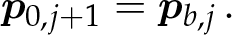
To define an arbitrary curve one could increase the order of the BB curve, but this may introduce numerical instability. A better approach for defining an arbitrary path is to compose it from a set of connected low-order curves. This also allows us to define additional properties at the joint points as shown in section 4.1. The connections should be carried out in way that achieves continuity of the curve and its derivatives up to some order. We consider three cases for joining two consecutive BB curves, demanding the continuity of the curve, continuity of the first order derivative and also continuity of the second order derivative. We describe how all these demands are related to the so-called tangential and angular velocities of the curve at the junctions. We denote two consecutive curves with r _j (λ) and r_j+1(λ), respectively. Here we allow the relative time to be dependent on the curve part t _j = Λ _j λ which gives us an additional degree of freedom. We also assume that the relative time t is reset to zero at the beginning of each BB curve.

To achieve continuity of a spline the following condition has to be met:

$$\underset{\lambda \to 1}{\lim }{r}_j\left(\lambda \right)=\underset{\lambda \leftarrow 0}{\lim }{r}_{j+1}\left(\lambda \right),$$

(55)

which yields the condition for selecting the first control point in the next curve part:

$$p_{0,j+1}=p_{b,j}.$$

(56)

This means that the curve is continuous, but the orientation of the tangent coming into the junction may or may not be the same as the one leaving the junction, ${\phi }_{b,j}\ne {\phi }_{0,j+1}.$ The same fact also applies to the tangential velocity $v_{b,j}\ne v_{0,j+1}$ , the angular velocity $w_{b,j}\ne w_{0,j+1},$ and the tangential acceleration $a_{b,j}\ne a_{0,j+1}.$

To achieve continuity of the BB spline up to the first order in addition to the condition (55) the following condition has to be met:

$$\frac{1}{{\mathrm{\Lambda }}_j^{}}\underset{\lambda \to 1}{\lim }\frac{\partial r_j\left(\lambda \right)}{\partial \lambda }=\frac{1}{{\mathrm{\Lambda }}_{j+1}^{}}\underset{\lambda \leftarrow 0}{\lim }\frac{\partial r_{j+1}\left(\lambda \right)}{\partial \lambda },$$

(57)

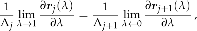
which yields an additional condition for selecting the second control point in the next curve part:

$$p_{1,j+1}=\left(\frac{{\mathrm{\Lambda }}_{j+1}}{{\mathrm{\Lambda }}_j}+1\right)p_{b,j}-\frac{{\mathrm{\Lambda }}_{j+1}}{{\mathrm{\Lambda }}_j}{p}_{b-1,j}.$$

(58)

Assume that the tangential velocity at the end point of the previous curve is not zero, v _b,j ≠ 0. Then, in addition to the continuous position, the orientation and tangential velocity are also continuous at the junction point, φ _b,j = φ_0,j+1 and v _b,j = v_0,j+1; but the angular velocity and tangential acceleration may still not be continuous at the junction point.

To achieve continuity of a spline up to the second order in addition to the conditions (59) and (57) the following condition has to be met:

$$\frac{1}{{\mathrm{\Lambda }}_j^2}\underset{\lambda \to 1}{\lim }\frac{{\partial }^2{r}_j\left(\lambda \right)}{\partial {\lambda }^2}=\frac{1}{{\mathrm{\Lambda }}_{j+1}^2}\underset{\lambda \leftarrow 0}{\lim }\frac{{\partial }^2{r}_{j+1}\left(\lambda \right)}{\partial {\lambda }^2},$$

(59)

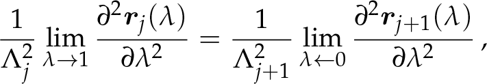
which yields an additional condition for selecting the third control point in the next curve part:

$$p_{2,j+1}={\left(\frac{{\mathrm{\Lambda }}_{j+1}}{{\mathrm{\Lambda }}_j}+1\right)}^2{p}_{b,j}-2\frac{{\mathrm{\Lambda }}_{j+1}}{{\mathrm{\Lambda }}_j}\left(\frac{{\mathrm{\Lambda }}_{j+1}}{{\mathrm{\Lambda }}_j}+1\right)p_{b-1,j}+\frac{{\mathrm{\Lambda }}_{j+1}^2}{{\mathrm{\Lambda }}_j^2}{p}_{b-2,j}.$$

(60)

In this case, in addition to the continuity of the position, orientation and tangential velocity, the angular velocity and tangential acceleration are also continuous at the junction point, ω_b,j = ω_0,j+1 and a_b,j = a_0,j+1.

4.3. Bernstein-Bézier curve under projective transformation

Since the perspective transformation of homography (4) is a non-linear transformation, the BB curve (41) cannot be transformed through homography from the world to image frame, or vice versa, in terms of the control points. However, the curve and also the curve's derivatives can be transformed from one frame to another, and the homography transformation does not break apart the continuity of the curve to the specific order, since the continuity and smoothness are properties of the curve that are invariant under homography transformation.

Since the Bernstein basis polynomials B_i,b(λ) form a partition of unity: ${\sum }_{i=0}^b{B}_{i,b}\left(\lambda \right)=1,$ the equation (41) does not change even if the points are defined in homogeneous coordinates. Applying the homography transformation (4) to the two-dimensional BB curve in the world frame $r_w^T\left(\lambda \right)=\left[r_x\left(\lambda \right)r_y\left(\lambda \right)1\right],$ , defined with the control points $p_i^T\left(\lambda \right)=\left[p_{x,i}{p}_{y,i}1\right],$ the BB curve in the image frame $r_p^T\left(\lambda \right)=\left[r_u\left(\lambda \right)r_v\left(\lambda \right)1\right]$ is as follows:

$$\begin{array}{l}{r}_u\left(\lambda \right)=\frac{{\sum }_{i=0}^b{B}_{i,b}\left(\lambda \right)h_1^T{p}_i}{{\sum }_{i=0}^b{B}_{i,b}\left(\lambda \right)h_3^T{p}_i},\\ r_v\left(\lambda \right)=\frac{{\sum }_{i=0}^b{B}_{i,b}\left(\lambda \right)h_2^T{p}_i}{{\sum }_{i=0}^b{B}_{i,b}\left(\lambda \right)h_3^T{p}_i}.\end{array}$$

(61)

It is clear that the rational expression (61) cannot be written in a polynomial form like (41), so the transformed BB curve (rational BB curve) cannot be written in terms of the control points in the transformed frame.

Two distinctive approaches can be used in the design of the reference trajectory. The reference trajectory can be designed in terms of the control points in the world plane, and then transformed into the image frame according to the equation (61). This approach requires knowledge of the homography matrix H , and if the homography matrix is not exactly known, there will be an inherent error that the controller will not be able to eliminate, since the control error is defined in the image space. An alternative is to define the trajectory in the image frame directly. The equations in section 4.1 and section 4.2 stay exactly the same, except that they are all defined in the image frame, and therefore all the values are expressed in pixels instead of metres. This is the preferred way, since the control error is also defined in the image space, and therefore there is no inherent error. In the previous approach the trajectory would need to be designed in the world plane, then transformed into the image plane and then inspected in the image frame to see if the transformation is accurate enough for the given task. In other words, no matter which approach is selected for generation of the trajectory, the trajectory should always be inspected in image space, but in the case where the trajectory is designed in the image space, this step is done inherently.

5. Experiments

We first tested the presented control algorithm in a simulation environment. The camera was positioned to some arbitrary location in space, in a way that the ground plane was in the camera's field of view. We defined the reference trajectory with the fifth order BB spline, and demanded from the trajectory to have continuous derivatives up to the second order — which means that the tangential and angular velocity are both continuous functions. We selected the time length of all the BB curves in the spline to be Λ = 5 s.

To the outputs of the system a normally distributed white noise with zero mean and a variance σ _n = 2 px² was added. The sampling time was selected to be T_s = 0.1 s. The system was supposed to have a delay of two samples. The initial tangential velocity in the dynamic feedback compensator was set to the tangential velocity at the beginning of the reference trajectory in the world space. The error model predictive controller was initialized with the following values:

$$Q=\left[\begin{array}{cc}1& 0\\ 0& 0.1\end{array}\right],R=\left[0.001\right],A_r=\left[\begin{array}{cc}0.65& 0\\ 0& 0.65\end{array}\right].$$

(62)

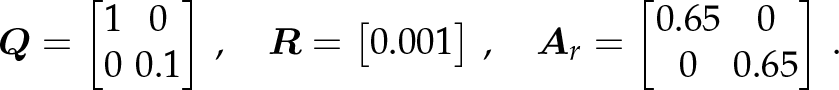
The Kalman filter was initialized with the following values of the covariance matrices:

$$N=\left[3\right],V=P=\left[\begin{array}{cc}0.05& 0\\ 0& 0.5\end{array}\right].$$

(63)

The robot was displaced from the starting location of the reference trajectory (non-zero initial condition).

With the selected parameters, we made several experiments. For the control performance assessment, we defined several performance evaluation functions:

$$\begin{array}{l}SSE=\sqrt{{\displaystyle \sum _{k=1}^K{e}_u^2\left(k\right)+e_v^2\left(k\right)}},\\ SAE={\displaystyle \sum _{k=1}^K\sqrt{e_u^2\left(k\right)+e_v^2\left(k\right)}},\end{array}$$

(64)

$$\begin{array}{l}SSd{U}_c=\sqrt{{\displaystyle \sum _{k=2}^K{\left(c\left(k\right)-c\left(k-1\right)\right)}^2}},\\ SAd{U}_c={\displaystyle \sum _{k=2}^K\left|c\left(k\right)-c\left(k-1\right)\right|},\end{array}$$

(65)

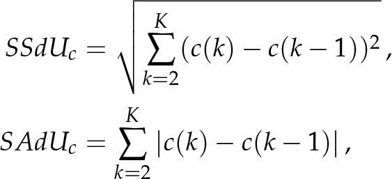
where e _u (k) = r _u (k) – u(k) and e _v (k) = r _v (k) – v(k), and c can be either v or ω. The criterion functions SSE and SAE evaluate the trajectory-tracking error, while the cost functions SSdU _c and SAdU _c evaluate the control effort.

Since the control algorithm demands knowledge of the homography (the mapping between the points in the image and world plane), we first evaluated the robustness of the proposed algorithm to an imprecise estimation of the homography matrix. The bold quadrilateral in Figure 3(b) shows the boundaries of the plane that are visible in the image, and the other ten thin quadrilaterals represent the estimated visible area in the image — each quadrilateral represents one homography. The performance of the tracking algorithm for all the inaccurately estimated homography matrices is depicted in the other three figures in Figure 3, and in table Table 1 some statistics about the control performance for all the cases is gathered.

Figure 3.

Trajectory-tracking (a) with respect to the imprecise estimation of the homography; (b) boundaries of the plane that are visible in the image for different estimations of the homography (quadrilateral with strong edges corresponds to the true homography); (c) extended inputs and (d) control inputs. In all the figures all ten signals are overlaid.

Table 1.

Evaluation of the trajectory-tracking performance with respect to the imprecise estimations of the homography.

	SSE	SAE	SSdU v	SAdU v	SSdU ω	SAdU ω
	px	px	ms−1	ms−1	s−1	s−1
Min	129.1	1094	0.1203	1.671	10.16	111.6
Mean	151.5	1505	0.183	2.085	11.87	120.2
Max	200.4	2519	0.3206	2.954	16.14	131.7

The model predictive control algorithm can be tuned in terms of the prediction horizon. To evaluate the influence of the prediction horizon h on the control quality, we considered cases where the prediction horizon takes values in the range from one to ten. The trajectory-tracking performance is evaluated in Table 2, and also shown in Figure 4 for the length of the prediction horizon one and five. The measurements were repeated twenty times. In this case we assumed that the homography matrix is known precisely.

Table 2.

Evaluation of trajectory-tracking performance with respect to different lengths of the prediction horizon h.

h	SSE	SAE	SSdU v	SAdU v	SSdU ω	SAdU ω
	px	px	ms−1	ms−1	s−1	s−1
1	270.1	2439	0.09405	1.344	4.64	37.36
2	129.5	1049	0.1724	2.042	14.34	148.3
3	179.4	1356	0.1054	1.493	5.644	57.62
4	147.2	1093	0.1245	1.66	7.746	83.08
5	132.4	988.7	0.1416	1.783	9.807	104.9
6	127.9	992.7	0.1566	1.902	11.88	122.8
7	127.8	1000	0.1644	1.975	12.74	132.9
8	129.3	1039	0.1685	2.028	13.85	143.5
9	130.2	1066	0.1721	2.047	14.01	146.3
10	130.4	1076	0.1752	2.058	14.07	147.5

Figure 4.

Trajectory-tracking (a), (c) for the length of the prediction horizon h = _{1 (top row) and h} = 5 (bottom row); (b), (d) control inputs. In all the figures all the signals from 20 repeats of the experiment are overlaid.

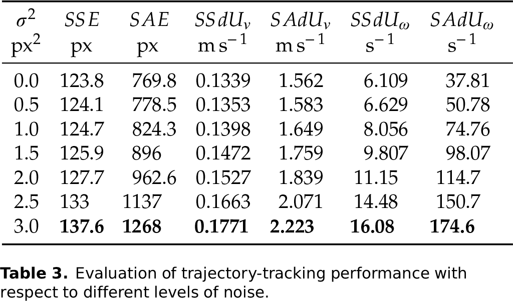
In all the experiments considered the output of the system was corrupted by white Gaussian noise of variance σ² _n = 2 px². Furthermore, we also evaluated the performance due to different levels of noise, and the results are gathered in Table 3. We again assumed that the homography matrix is precisely known. Figure 5 shows reference-tracking in a case where the level of the noise is σ² _n = 3 px², and this figure can be compared to Figure 4(c), Figure 4(d) where the value of noise is σ² _n = 2 px², but other simulation conditions are the same.

Table 3.

Evaluation of trajectory-tracking performance with respect to different levels of noise.

σ2	SSE	SAE	SSdU v	SAdU v	SSdU ω	SAdU ω
px2	px	px	ms−1	ms−1	s–1	s–1
0.0	123.8	769.8	0.1339	1.562	6.109	37.81
0.5	124.1	778.5	0.1353	1.583	6.629	50.78
1.0	124.7	824.3	0.1398	1.649	8.056	74.76
1.5	125.9	896	0.1472	1.759	9.807	98.07
2.0	127.7	962.6	0.1527	1.839	11.15	114.7
2.5	133	1137	0.1663	2.071	14.48	150.7
3.0	137.6	1268	0.1771	2.223	16.08	174.6

Figure 5.

Trajectory-tracking (a) with respect to different levels of noise; (b) control inputs. In all the figures all the signals from 20 repeats of the experiment are overlaid.

To test the performance of the tracking controller on the real system, we implemented a simple image-tracking algorithm. To simplify the image-based robot tracking, we equipped a robot with a colour marker that can be recognized easily by the image recognition system [7]. The position of the robot is supposed to be at the centre of the largest detected patch. The recognized robot in the image is shown in Figure 6(a). In Figure 6(b) the results of the trajectory-tracking on the real system are presented. To improve readability, only every fifth sample in Figure 6(b) is marked with a symbol, and all the samples are connected with a line.

Figure 6.

Trajectory-tracking on a real robot: (a) view from the camera with the detected robot and (b) trajectory-tracking results in the image frame.

6. Conclusion

We presented the design of a visual controller for trajectory-tracking of a mobile robot that is observed by an overhead camera that can be placed at arbitrary inclination with respect to the ground plane. An image-based visual servoing principle was used in the design of the control algorithm. The presented algorithm includes a Kalman filter for state estimation and a model predictive control for reference-tracking. Since the proposed control algorithm requires a special trajectory that is at least twice differentiable, we gave an extensive description for the use of Bernstein-Bézier curves to tackle the trajectory design problem. The presented control algorithm was designed in the discrete-time space.

The control algorithm was derived assuming the homography H is precisely known, but actually it can only be estimated with finite precision in the process of calibration. Nevertheless, the experimental results in Figure 3 and Table 1 show that the control algorithm is robust to imprecise estimation of the homography.

Another important parameter of the control algorithm is the length of the model predictive control horizon h. The evaluation of reference tracking performance with respect to the length of the prediction horizon (Figure 4 and Table 2) shows that good tracking performance is not achieved when the control horizon is only of unit length. When we increase the length of the control horizon the tracking performance improves, but too long a control horizon may smooth the trajectory sharp turns more than is desirable. The longer control horizon also increases the control high-frequency gain (Figure 4(d)). In our case, the control horizon of length five seems to give good trade off between tracking performance and the control gain (Table 2).

The measured position of the robot in the image, obtained by the image-tracking algorithm, is inherently corrupted with noise. The experimental results in Figure 5 and Table 3 show the influence of the noisy measurements on the trajectory-tracking performance, and confirm that the controller is robust to noise.

The simulation experiments as well as experiments made on the real system (Figure 6) confirm that the presented control approach is suitable for solving the trajectory-tracking task. The results prove the applicability of the presented control design, even in the case of non-ideal conditions.