Top-View-Based Guidance for Blind People Using Directional Ellipse Model

Abstract

The guidance system proposed in this paper aims to complement the white cane by monitoring road conditions in a medium range for blind pedestrians in real time. The system prototype employs only one webcam fixed at the waist of user. One of the main difficulties of using a single camera in outdoor obstacle detection is the discrimination of obstacles from a complex background. To solve this problem, this paper re-formulates top-view mapping as an inhomogeneous re-sampling process, so that background edges are sub-sampled while obstacle edges are oversampled in the top-view domain. Morphology filters are then used to enhance obstacle edges as edge-blobs, which are further represented using a directional ellipse as a new model for obstacle classification. Based on the identified obstacles, safe walking area is estimated by tracking a polar edge-blob histogram. To transfer the information obtained from image domain to language domain, this paper proposes a verbal message generation scheme based on fuzzy logic. The efficiency of the system is confirmed by testing the system with visually impaired people on outdoor pedestrian paths.

1. Introduction

Autonomous mobility is of extreme importance for visually impaired people, and white canes are their primary tools when travelling independently. However, white canes are very limited in sensing the environment. Therefore, considerable efforts have been made over the last 20 years to complement the white cane with various types of electronic guidance systems able to detect obstacles at a greater range.

1.1 Related work

These guidance systems can be categorized according to how the information is gathered from the environment and delivered to the blind user [2]. In general, information can be gathered with ultrasonic sensors [3], laser scanners [4], or cameras, and users can be informed via auditory [5] or tactile sense [6, 7]. In recent years, camera-based systems have won much attention due to advantages like large sensing area, rich sensing data and low cost. Most existing vision-based guidance systems use stereo-vision methods. In these systems, stereo cameras are used to create a depth map of the surrounding environment, and then this depth map is transformed into stereo sound or tactile vibration. For instance, Mora [5] developed a navigation device to transform a depth map into a stereo sound space. Meanwhile, the TVS [6] and Tyflos [7, 8] navigator systems convert a depth map into vibration sensing on a 2-D vibration array attached to the user's abdomen. The ENVS system [9] transforms a depth map into electrical pulses that stimulate the nerves in the hand's skin.

In addition to stereo-vision systems, systems using only a single camera have also been proposed. The single camera system is more compact and easier to maintain. Some of these mono-vision systems focus on identification of object pixels among background pixels. For example, in the NAVI system proposed by Sainarayanan et al. [10], a fuzzy learning vector quantization (LVQ) neural network is trained for the classification of object pixels and background pixels. Then, the object pixels are enhanced and the background pixels are suppressed. Although the classification rate in an indoor environment is promising, the LVQ classifier is trained assuming that backgrounds are of lighter colour than obstacles, which may not always hold in outdoor environment applications.

1.2 Outline of the proposed method

As we have seen, many blind guidance systems, using stereo or monocular vision systems, have been successfully tested in indoor environments [2]. However, very few have been reported to be equally highly effective in outdoor scenarios with complex backgrounds. The main contribution of this paper is a monocular edge-feature-based approach for obstacle detection and avoidance in complex outdoor environments.

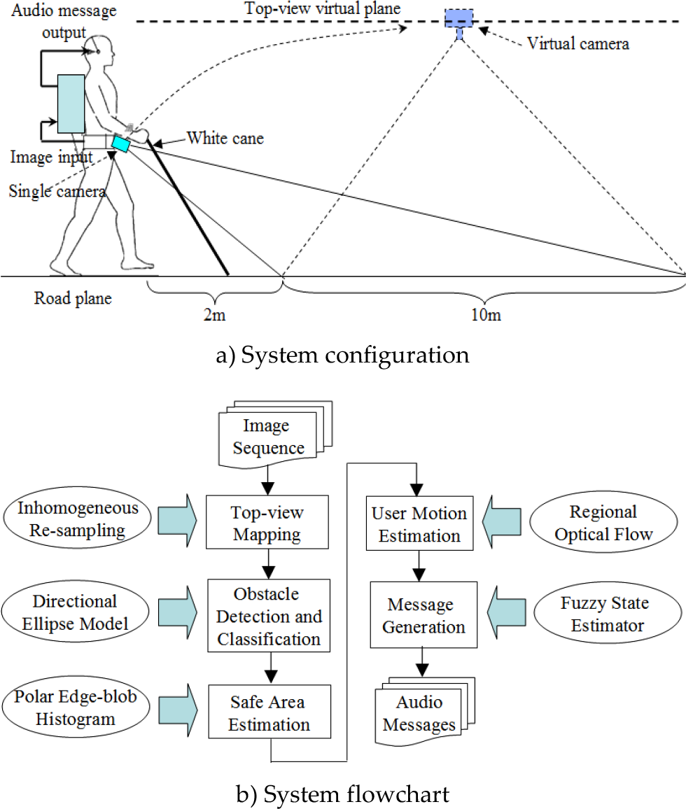
An overview of the system is illustrated in Figure 1. In the proposed system, a camera is attached to the blind user's waist and angled slightly downward towards the road in front. As shown in Figure 1a, the white cane still acts as a reliable tool covering a close range of up to 2 metres in front of the user, with the downward-looking camera acting as a complementary sensor covering a medium range of about 10 metres. With this configuration, the white cane can be used to detect ground-level obstacles and holes in the near field, while the camera looking a further distance ahead can provide useful information like safe walking direction and obstacle locations and numbers.

Figure 1.

System overview

In contrast to Sainarayanan's method, which uses pixel-wise features, edge-based features are explored to discriminate obstacles from a complex road pavement background. By re-sampling the original image inhomogeneously and mapping it onto a top-view virtual plane, pavement edges in the near field are sub-sampled, while obstacle edges in the far field are over-sampled. Morphology filters are then used to enhance this inhomogeneous re-sampling effect on connectivity and scale of edges, so that enhanced obstacle edge-blobs can be distinguished. To further classify obstacles, a directional ellipse model is built for edge-blobs on the top-view plane. Finally, information regarding obstacles, safe area and user motion is converged at the message generation engine, where a fuzzy state estimator is designed to determine what types of messages should be generated and when to deliver them to the user.

2. Obstacle Detection on Top-view

2.1 Inhomogeneous Top-view Re-sampling and Mapping

Top-view mapping is an inhomogeneous re-sampling process that has been widely used in applications like lane detection, mainly for the purpose of road geometry recovery. Some researchers have also attempted obstacle detection on top-view images. The basic idea is to generate a difference image by associating two top-view images either spatially [11] with a stereo camera or temporally via a single camera [12]. On this difference image, planar patterns like road textures are removed, while high objects like vehicles are retained in the form of large clusters of non-zero pixels with a specific shape. While this approach is effective to detect vertical obstacles like vehicles on a highway, problems emerge when it comes to blind navigation in an urban environment. First, ground-level obstacles are removed on the difference image, which could be dangerous for the blind pedestrian. Second, due to the low-speed, forward-rolling motion of pedestrians, an obstacle's blob patterns may not be prominent enough to identify them against noise on a temporal correlated difference image. In this paper, rather than using a difference image, the effects of top-view re-sampling and mapping on obstacle edges are studied, and several useful properties are modelled for the identification of obstacle edges in background clutters. In this section, this re-sampling process is re-formulated in horizontal and vertical directions, and its effect on the scale and connectivity of edges is discussed.

The model of vertical direction re-sampling is illustrated in Figure 2a. In Figure 2a, C_r is the real camera centre with S_r as its image plane, while C_v is the virtual top-view camera centre with S_v as the virtual top-view plane. To figure out the re-sampling relationship between the S_r and S_v planes, the only parameters that are required are ϕ and θ. According to the geometrical description in Figure 2a, for each point P_v on the virtual top-view plane S_v, the corresponding sampling point P_r on the real image plane S_r can be calculated based on the common projection point P_g on the ground plane. As (1) shows, for each point i on the top-view plane, the corresponding sampling point h on the real image plane can be obtained:

Figure 2.

Top-view re-sampling model

$$\begin{array}{l}{X}_1=H_c\cdot \tan \varphi ,X_2=H_c\cdot \tan (\theta +\varphi )\\ X_3=X_2-X_1,X_s=i\cdot X_3/H_T(i=0\dots H_T)\\ \gamma =\arctan [(X_1+X_s)/H_c]-\varphi \\ h=\{\begin{array}{c}{H}_I/2-f\cdot \tan (\theta /2-\gamma )(\gamma \le \theta /2)\\ H_I/2+f\cdot \tan (\gamma -\theta /2)(\gamma >\theta /2)\end{array}\end{array}$$

(1)

The model of horizontal re-sampling is illustrated in Figure 2b: the length of each row W_k in C _r 's field of view on the ground plane can be calculated according to the triangular similarity; also, by comparing W_k with C _v 's field of view on the ground plane the sampling ratio can be computed, as in (2):

$$\begin{array}{l}{W}_G=X_3\cdot (W_T/H_T),X_k=X_1+X_s\\ W_k=W_G\cdot X_k/X_2,W_{k\_p}=W_k\cdot (W_T/W_G)\\ W_s=W_T/W_{k\_p}\end{array}$$

(2)

Figure 3 shows the re-sampling graph in the vertical and horizontal directions. These graphs are obtained by applying (1) to an image with size 320×240, with the origin sets at the lower-left corner of the image plane. Figure 3a shows the re-sampling rate in the vertical direction. This indicates how many rows of the original image are encoded by each row of the top-view image: more than 1 means sub-sampling, while smaller than 1 means over-sampling. Figure 3b shows the horizontal re-sampling rate for each row of the top-view image, which represents how many pixels need to be jumped over to sample one pixel in each row of the original image. It turns out that the re-sampling rate decreases from the bottom to the top row.

Figure 3.

Top-view re-sampling graph

Figure 4 shows a comparison between the vertical edge map on an original image and a top-view image. On the original image edge map, it is very difficult to discriminate the obstacle edges because of the pavement edges. However, on the top-view edge map, the obstacle edges are enhanced by oversampling while the pavement edges are suppressed by sub-sampling.

Figure 4.

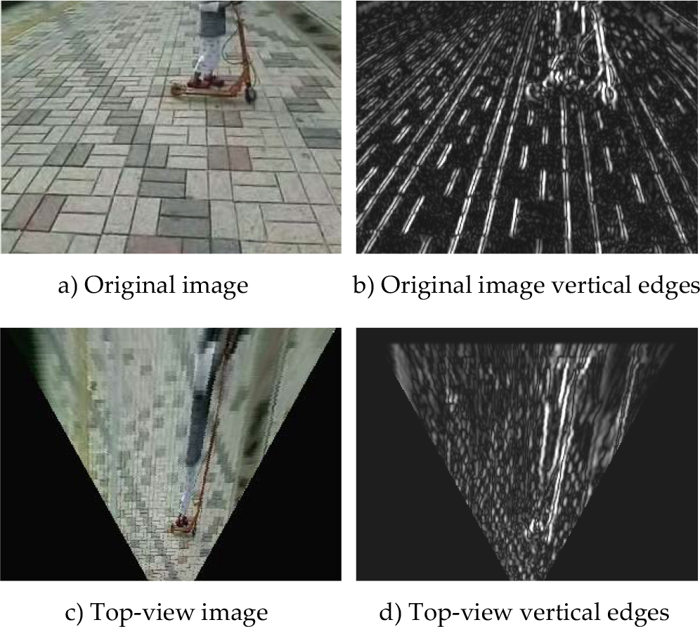
Top-view re-sampling effect on vertical edges

2.2 Edge-blob Extraction

After top-view re-sampling has enhanced the obstacle edges in scale and connectivity, a combination of morphology operations and connected component analysis is used to extract edge-blobs with large size. These edge-blobs are regarded as candidate obstacle representations. On the top-view image, road texture is re-constructed so that sub-sampled pavement edges appear as small vertical segments with similar size. This makes it easy to remove those small edge segments using fixed-size morphological filters. Here, a 3×3 rectangular structure element is used to remove pavement edge segments with an opening operation, followed by a closing operation to fill the gaps. A connected component-labelling operation is then applied to group the connected foreground pixels into blobs. Blobs with size smaller than a pre-defined threshold are discarded. As shown in Figure 5c, many small edge-blobs from the pavement are eliminated. Finally, as shown in Figure 5d, only two major edge-blobs are selected, which correspond to possible obstacle regions. As mentioned in section 2.1, since top-view re-sampling sub-samples the original image in the horizontal direction, obstacle width will shrink in the top-view domain. This property makes it easier for edge-blobs to fill up the whole obstacle region in the top-view domain. Therefore, these edge-blobs can be used as a kind of obstacle representation on the top-view plane.

Figure 5.

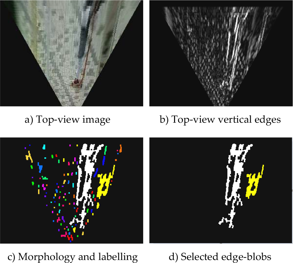
Edge-blob extraction

2.3 Directional Ellipse Model

This paper proposes a directional ellipse model for discrimination of vertical and planar type obstacles, and the properties of the edge-blob feature on the top-view domain are further explored in this section. Vertical obstacles are defined here as obstacles that rise significantly above the road plane, like trees, poles, and other pedestrians. These vertical obstacles usually have vertical edges in the original-view domain. Planar obstacles are those lower obstacles that are close to the road plane, like road-side curbs and stairs; these obstacles usually have significant edges along the road direction in the original view. In the top-view domain, obstacles can also be characterized by their distinct edge orientations, although the edge orientation feature is different to that in the original view domain. This is illustrated in Figure 6: C_r is the real camera's optical centre and S_r is the real camera's image plane, while C_v is the top-view virtual camera's optical centre and S_v is the top-view virtual plane.

Figure 6.

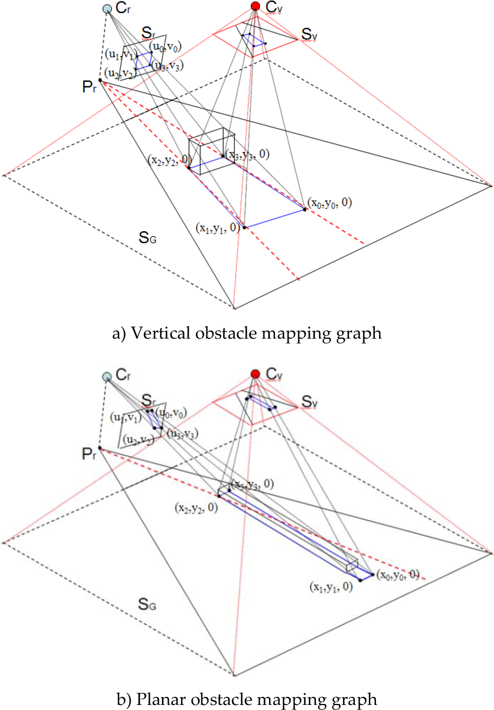
Mapping of obstacle to the top-view plane

In Figure 6a, a vertical obstacle is mapped to the S_r plane through central projection, with the vertical edges still appearing vertical. During the top-view mapping process, the obstacle's image on the S_r plane is mapped to the S_v plane, which is parallel to the ground plane S_G. As a result, on the S_v plane, the horizontal edges of the obstacle still appear horizontal, but the vertical edges are stretched toward point P_r, which is the perpendicular projection of C_r on the ground. It can be observed that, through top-view mapping, vertical lines in the original image are mapped to lines passing through the same point in the top-view domain. This vertical line distortion can be partly explained by the inhomogeneous re-sampling process discussed in section 2.1; it can also be derived from an IPM (inverse perspective mapping) formula [11].

In (3), the point on the real image plane S_r is represented by (u, v), and the point on the ground plane S_G is represented by (x, y, 0). Vertical lines on the image plane S_r can be represented by v = k, where k is a constant value; substituting this into (3), we can get (4), where c₁ and c₂ are constant terms. Finally, we can obtain (5), where (l. d) represents the camera centre's projection point P_r on the ground plane.

$$\{\begin{array}{l}x(u,v)=h\times \cot [(\theta -\partial )+u\frac{2\partial }{n-1}]\times \cos [(\gamma -\partial )+v\frac{2\partial }{n-1}]+l\\ y(u,v)=h\times \cot [(\theta -\partial )+u\frac{2\partial }{n-1}]\times \sin [(\gamma -\partial )+v\frac{2\partial }{n-1}]+d\end{array}$$

(3)

$$\{\begin{array}{l}x=h\times \cot [(\theta -\partial )+u\frac{2\partial }{n-1}]\times c_1+l\\ y=h\times \cot [(\theta -\partial )+u\frac{2\partial }{n-1}]\times c_2+d\end{array}$$

(4)

$$y-d=(c_2/c_1)(x-l)$$

(5)

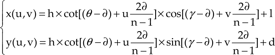
In Figure 6b, the shape of the planar obstacle will appear in a perspective effect on the original image plane S_r. However, when mapping to the top-view plane S_v, its original shape is retained. It can be observed that edges from planar obstacles lie along a different direction with respect to P_r's radial direction, which is represented by the red dash line on the S_G plane. This distinct edge distribution feature can be used to discriminate vertical obstacles from planar ones in the top-view domain. Therefore, it is important to model obstacle edge orientation in a robust way. Here, an ellipse model is used to model edge-blobs that are extracted in the top-view domain.

As Figure 7 shows, an ellipse is calculated to bound the points contained in each edge-blob. The ellipse can be specified by a set of geometric parameters –: <(x₀, y₀), R_a, R_b, θ > – which can be used to describe the spatial distribution of the blob points. The major axis orientation θ is calculated using central moment u_p,q of the blob, which depicts the direction along which the largest variation occurs. Here, this major axis orientation is defined as the direction of the ellipse. The geometric parameters in this directional ellipse model can be calculated using (6).

Figure 7.

Directional ellipse model definition

$$\begin{array}{l}{x}_0=\frac{1}{N}{\displaystyle \sum _{i=1}^N{x}_i{y}_0=}\frac{1}{N}{\displaystyle \sum _{i=1}^N{y}_i}\\ {\mathrm{u}}_{\mathrm{p},\mathrm{q}}={\displaystyle \sum _{\mathrm{i}=1}^{\mathrm{N}}}{\left({\mathrm{x}}_{\mathrm{i}}-{\mathrm{x}}_0\right)}^{\mathrm{P}}\cdot {\left({\mathrm{y}}_{\mathrm{i}}-{\mathrm{y}}_0\right)}^{\mathrm{q}},\theta =\frac{1}{2}\cdot {\tan }^{-1}[\frac{2u_{11}}{u_{20}-u_{02}}]\\ R_a=(u_{20}+u_{02})/2+\sqrt{{(u_{20}+u_{02})}^2/4-u_{20}\cdot u_{02}+u_{11}{}^2}\\ R_b=(u_{20}+u_{02})/2-\sqrt{{(u_{20}+u_{02})}^2/4-u_{20}\cdot u_{02}+u_{11}{}^2}\end{array}$$

(6)

2.4 Obstacle Classification

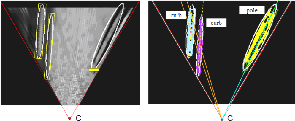
The directional ellipse model provides new region features for obstacle type classification. One of the most important features is defined as Deviation from Radial Orientations (DRO). In section 2.3, it has already been proved that, in the top-view domain, the vertical obstacle's edges should lie along the radial directions with respect to point P_r, while the planar obstacle's edges should deviate from this radial direction. In other words, the deviation of a fitted directional ellipse from the corresponding radial direction can be used to evaluate the likelihood of its becoming a vertical obstacle.

$$D(i)=|{\tan }^{-1}[\frac{y_{0i}-y_c}{x_{0i}-x_c}]-{\theta }_i|$$

(7)

As illustrated in Figure 8, the radial direction of a given directional ellipse is defined as the direction of the line passing through the convergence point C and the centre point of this ellipse, while the direction of the ellipse itself is described by the direction of its major axis. The difference between an ellipse's radial direction and its major axis direction is defined as Deviation from Radial Orientations DRO. DRO measurement is calculated as in (7), where (x_0i, y_0i) is the centre point of ellipse i, (x_c, y_c) is the convergence point, and θ_i is ellipse i's major axis direction angle. To train a classifier based on this DRO feature, thousands of sample images are collected from different pedestrian path scenes. In the top-view domain, the directional ellipse fitting based on edge-blobs simplifies the labelling and learning process. The manual interaction is only required for the labelling of the directional ellipse as positive (vertical obstacles) or negative (planar obstacles). Here. vertical obstacle means any high obstacle with quasi-vertical edges, like trees, poles, and pedestrians, while planar obstacle means any ground-level obstacle with edges along the road, like road curbs, fence curbs, and stairs. The DRO values obtained from the training data are shown in Figure 9.

Figure 8.

Deviation from radial orientations

Figure 9.

DRO training set

It can be observed from Figure 9 that the DRO values of the two classes overlap due to noise data introduced at the ellipse-fitting stage. Therefore, a soft-margin SVM classifier is trained to deal with the noise. The classification function is expressed in (8): given a training data set D={(x_i, y_i), i=1…N}, where x_i ∊R, y_i∊{−1, 1}, a soft-margin decision plane can be calculated by minimizing the evaluation function in (9), where C is a cost parameter which tunes the trade-off between the size of the margin and the size of the error measured by ξ_i.

$$f(x)=\mathrm{si}gn(w^{\ast }{}^T\cdot x-b^{\ast })$$

(8)

$$L(w,\xi )=\frac{1}{2}||w|{|}^2+C{\displaystyle \sum _{i=1}^N{\xi }_i}$$

(9)

After the DRO values have been examined to classify obstacles into vertical and planar types, shape properties of the ellipse like anisometry, a = R_a/R_b, and bulkiness, b = πR_aR_b/S, are employed to further classify obstacles into four types, as shown in Figure 10.

Figure 10.

Obstacle types classification

Poles and curbs are obstacles with a long and thin shape, with high anisometry and low bulkiness. Blocks and piles are obstacles with bulky shape, low anisometry and high bulkiness. Poles are thin vertical obstacles including pedestrians. Curbs are thin planar obstacles including road-side curbs and stairs. Blocks are large vertical obstacles like buildings or other large objects on the road, while piles correspond to bulky planar obstacles like bushes, big stones or holes. Another SVM classifier is trained to carry out this shape classification.

3. Safe Area and User Motion Estimation

3.1 Polar Edge-blob Histogram

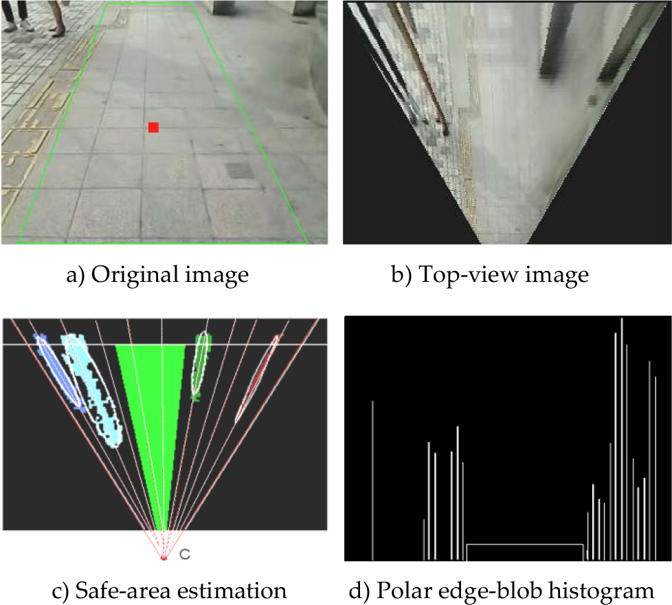
Based on the detected obstacles, a polar edge-blob histogram is constructed on the top-view image for the estimation of the safe walking area.

As shown in Figure 11c, on the edge-blob image, from the right boundary to the left boundary, radial directions (marked red dashes) are sampled with respect to the convergence point C. For each sampled radial direction, the number of edge-blob pixels that lie along this direction is counted. By accumulating all the sampled radial directions, a polar edge-blob histogram can be constructed as shown in Figure 11d. In the polar edge-blob histogram, the horizontal axis represents sampled radial directions in angles, and the vertical axis is the number of edge-blob pixels that lie along each sampled direction angle. The bins with high values indicate the directions where obstacles appear, while bins with zero values correspond to the directions where no obstacles exist. Therefore, the safe area should be estimated by the bins with zero values.

Figure 11.

Safe-area estimation using polar edge-blob histogram

3.2 Polar Edge-blob Histogram Tracking

Since the camera is attached to the user's waist, the camera will show some swing motions due to the gait of the human body. These swing motions will appear as noise added to the safe area positions. To estimate the safe area more steadily, the largest valley position on the polar histogram should be tracked.

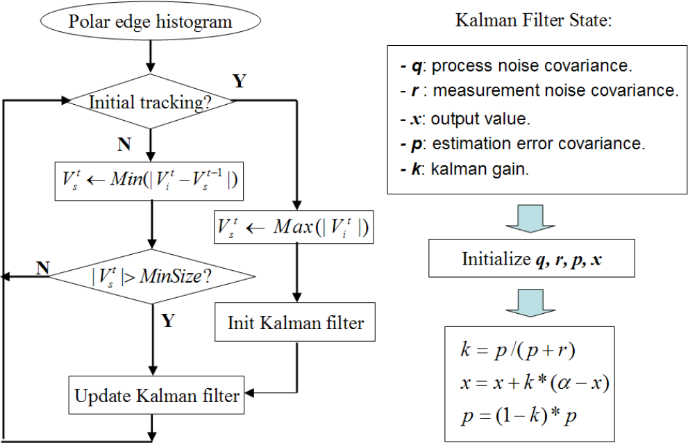
A flowchart of polar edge-blob histogram tracking is shown on the left side of Figure 12. For tracking initialization, consecutive zero-value bins in frame t are grouped as V^t_i and sorted according to their group size | V^t_i |. Then the largest bin group Max(| V^t_i |) is selected as the tracking group V^t_s in frame t . In the following frame, the zero bin group V^t_i, which is closest to the tracking group V^t–1_s in frame t-1 is selected as the tracking group | V^t_s | in frame t . If the size of tracking group | V^t_s | is smaller than a threshold, then tracking will be stopped and re-initialized from the beginning.

Figure 12.

Flowchart of polar histogram tracking

In addition to tracking on the polar edge-blob histogram, the polar angles of the safe-area boundaries in the top-view domain are also tracked by means of a Kalman filter. The tracking group V^t_s can be represented by two bounding direction angles: < α^t_l, α^t_r >, where α^t_l is the left bounding direction angle and α^t_r is the right bounding direction angle.

The blue curve in Figure 13 shows the measured value of α^t_r; this noisy value pattern is mainly caused by the camera's shaking motion with the user's rolling gait. The noise involved in this pattern can be approximated by Gaussian noise. Therefore, one-dimensional Kalman filters are used to find the stable estimation of < α^t_l, α^t_r >. The Kalman filter state variables are shown on the right of Figure 12. After initializing these state variables, the value of error covariance p and output value x are updated using the equations in Figure 12. The filtered output value of α^t_r is shown by the red curve in Figure 13.

Figure 13.

Kalman filtering result

3.3 User Motion Estimation

Since the camera is mounted on the waist of user, the camera's motion can be used as an approximation for the user's walking motion. In top-view image sequences, the movement of ground pixels can be regarded as an approximation of the user's walking motion projected on the top-view plane. As the ground pavement structure is reconstructed by top-view mapping, it would be very convenient to calculate the movement of ground pixels in the top-view domain. To calculate ground pixel movements, a KLT (Kanade-Lucas-Tomasi) tracker is used to track ground pixels through top-view image frames. As is shown in Figure 14, after obstacle edge-blobs are extracted, their corresponding directional-ellipse region can be cropped from the top-view image domain, so that only ground areas remains.

Figure 14.

Ground pixel tracking

The KLT tracker is then applied to the ground area to select ground feature points and track them through image frames. The user's walking motion projected on the top-view plane can be decoupled into translational motion and rotational motion. Define R as the rotation matrix and T as the translation matrix; these can be calculated by (10):

$$F_i=R{Q}_i+T+E_i(i=1,2,\dots n)$$

(10)

where F and Q are the corresponding feature locations in adjacent frames, and E is estimation error term. To find the optimized values for R and T , the weighted sum of squared error term in (11) should be minimized. Here the weight w_i is set using the largest eigenvalue of the inverse Hessian matrix for each selected feature point. The final solution for R and T is used as an approximation for the user's walking motion, based on which the user's walking speed and direction can be estimated.

$${\displaystyle \sum _{i=1}^n{w}_i}||E_i|{|}^2={\displaystyle \sum _{i=1}^n{w}_i}||F_i-R{Q}_i-T|{|}^2$$

(11)

4. Audio Message Generation

4.1 Guidance States Estimation

The message generation module works as a kind of human-machine interface between the guidance system and the blind user. The task of this module is to transform the information obtained from the image domain to the language domain, and deliver the right messages to the user at the right time. For the user feedback scheme, stereo sound and tactile arrays are also widely used. However, extensive training is required to enable the user to perceive the sound and vibration pattern. Verbal message feedback can provide semantic information in a more user-friendly way. Here, a message generation scheme using a fuzzy logic approach is proposed.

As shown in Figure 15c, the key idea of this message generation scheme is guidance states estimation. Here the guidance state is defined as a fuzzy variable, GS , with three modes: safe, normal and danger. For each mode, a related message set is defined with the type of messages most suitable for this mode. To estimate this state, four state variables are defined from the information obtained in the image domain. The first is obstacle density, d , which is defined as the ratio of obstacle areas with respect to the whole image area. This state variable is used to indicate the congestion of the road environment. The second variable is nearest obstacle, λ, which is defined as the vector pointing to the ground position of the nearest obstacle. The third variable is deviation from safe direction, α , defined as the difference between the user's walking direction and the recommended safe direction. The fourth variable is user's walking speed, v , which is calculated in pixel/frame. These four variables constitute a state vector < d , λ, α, v > for state evaluation. Figure 15b illustrates the definition of these four state variables.

Figure 15.

Fuzzy instruction generation scheme

As Figure 15c shows, the guidance modes are determined by the combination of the state variables. However, the relationship between the state variables and guidance modes is rather vague. To deal with this vagueness, a fuzzy logic model is proposed here. Membership functions of fuzzy subsets are introduced to model the state variables. A bell-shape membership function is used, as defined in (12). The membership function u_A(x) , associated with fuzzy set A , is represented by reference function L for the left part and R for right part; m is the mean value of A , and α< and β are the left and right spread of A . The L function in (13) is used, where p is the slope of fuzzy set A . Figure 16 shows the membership function u_d(x) of fuzzy subsets of state variable d ; the membership functions u_λ(x), u_α(x) and u_v(x) are similar.

Figure 16.

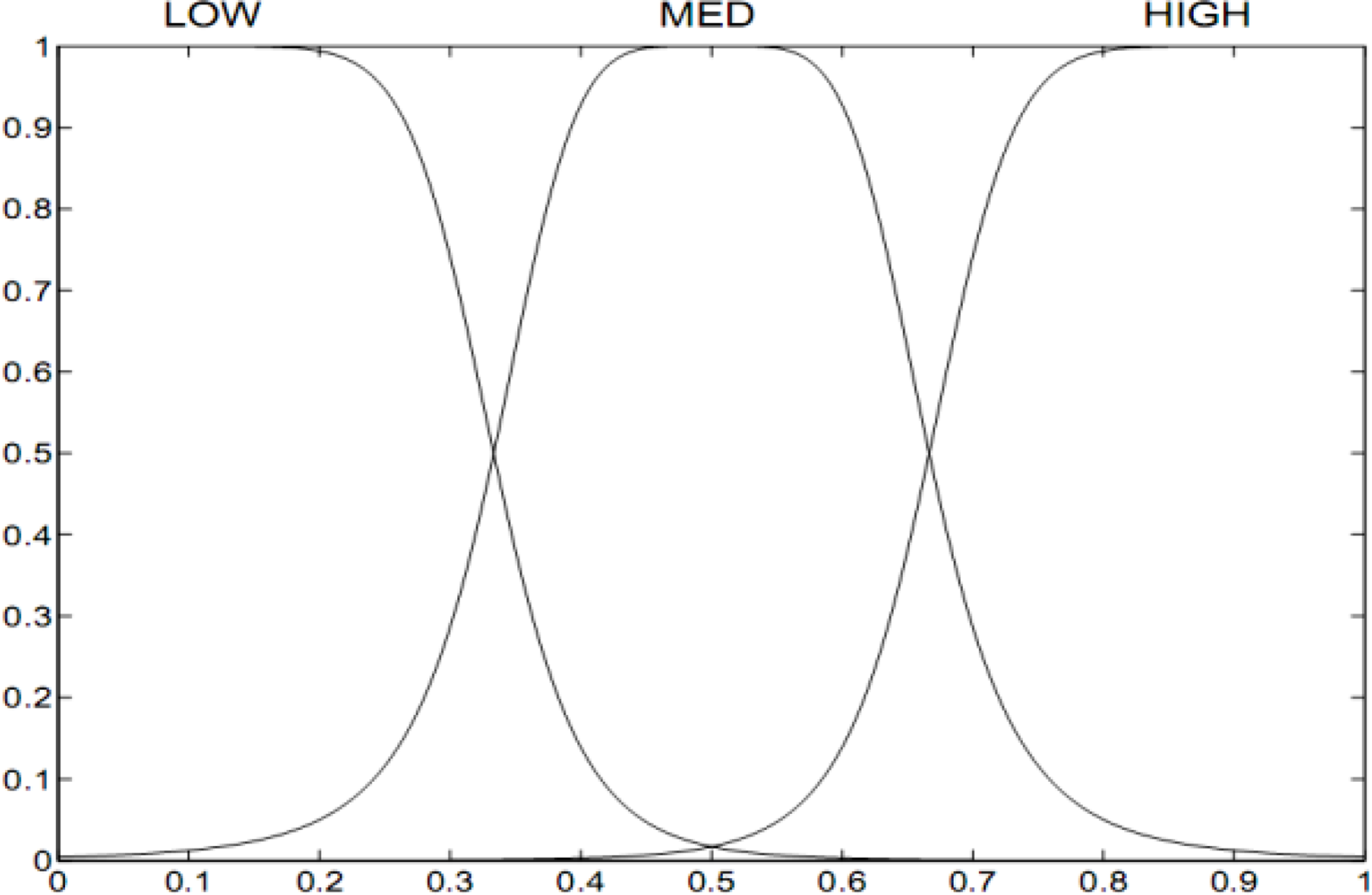
Membership functions of state variable

Figure 17.

Multimodal information transformation

$$u_A(x)=\{\begin{array}{c}L(\frac{m-x}{\alpha })forx\le m\\ R(\frac{x-m}{\beta })forx\ge m\end{array}$$

(12)

$$L(x)=\max (0,1-x^{-2p})=e^{-x^{2p}}$$

(13)

After introducing the membership functions of fuzzy subsets, linguistic variable terms can be used to describe the guidance process as follows: LOW is “low”, MED is “medium”, HIGH is “high”, S is “safe”, N is “normal” and D is “danger”. Then, a set of rules are defined as fuzzy conditional statements, for example: “If d is LOW and λ is LOW and α is LOW and v is LOW then GS is S”. The min-max compositional inference mechanism is used to derive fuzzy statements from the observed measurements of the state variables. In the max-min composition fuzzy inference method, the min operation is used for the AND conjunction (set intersection) and the max operation is used for the OR disjunction (set union) in order to evaluate the grade of membership of the antecedent clause in each rule. Table 1 shows some of the fuzzy rules derived and used by the system.

Table 1.

Some fuzzy rules derived and used by the system

No.	d	λ	α	v	GS
1	LOW	HIGH	ANY	ANY	S
2	HIGH	LOW	ANY	ANY	D
3	MED	HIGH	ANY	ANY	N
4	HIGH	MED	ANY	ANY	N
5	LOW	MED	ANY	ANY	S
6	MED	LOW	ANY	ANY	D
7	MED	MED	ANY	ANY	N
8	LOW	LOW	LOW	LOW	S
9	LOW	LOW	HIGH	ANY	N
10	LOW	LOW	ANY	HIGH	N
11	LOW	LOW	LOW	MED	S
12	LOW	LOW	MED	LOW	S
13	LOW	LOW	MED	MED	N
14	HIGH	HIGH	LOW	LOW	N
15	HIGH	HIGH	HIGH	ANY	D
16	HIGH	HIGH	ANY	HIGH	D
17	HIGH	HIGH	LOW	MED	N

4.2 Guidance Messages Generation

By applying the above monocular vision algorithms to the top-view image, three types of necessary information for guidance can be obtained: safe walking direction, obstacle positions, and user's walking motion. The next important step is to transform the information obtained from the image domain to the language domain, and deliver the verbal messages to the user in an appropriate manner.

The message generator works with the fuzzy state estimator discussed in the previous section. It determines the message sets that are most suitable to be delivered to the user in the current state, and filters out other less necessary messages. The filtering rules are defined as shown in Table 2. In the “Danger” state, a safe walking direction message must be acquired instantly, while in the other states it is more necessary to report obstacle positions in the surrounding environment in order for users to be able to maintain a safe walking direction by themselves.

Table 2.

Guidance Message Generation Rules

Guidance state	Output message set
Safe	safe direction, user motion close obstacle positions
Normal	safe direction, user motion, nearest obstacle position
Danger	safe direction, user motion

A message set example is shown in Table 3. The words in brackets are template words which can be changed according to the detection result. Object types are classified into vertical types (including poles and blocks) and planar types (including curbs and piles), as discussed in section 2.4. Rather than using metres to report distance, the number of average steps is used to enable more intuitive cognition. In the user motion set, the message “Large departure attention” is given when the user deviates too far from the safe direction. If user speed is too fast in danger mode, “Please slow down” will be prompted. On the other hand, if the user moves too slowly in safe mode, the system can also suggest that the user walks faster. If there are too many obstacles ahead, and insufficient safe space can be detected, the “stop” message may be delivered.

Table 3.

Verbal message example

Message type	Message example
Safe direction	Go (12 o'clock)
Obstacle position	(Poles) at (1 o'clock) (5 steps)
User motion	(Large departure) attention! Please (slow down/walk faster/stop).

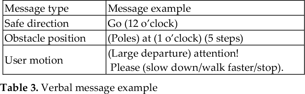
As Figure 18 shows, clock-face directions are used to give direction messages. Clock-face directions are broadly accepted as a common way to indicate directions for blind people. The estimated free path is mapped from the top-view domain (Figure 16a) to the original-view domain (Figure 16b), which is divided by projecting the top-half clock-face area (10 o'clock ∼ 2 o'clock) onto the centre horizontal line in the original image space. The centre of the mapped free path on the centre line is defined as the safe direction indicator. The clock-face section into which it falls determines the safe direction to be suggested to the user. Detected obstacle directions are also delivered in this way after mapping to the original image.

Figure 18.

Clock-face directions

Another important factor that affects guidance performance is the timing of guidance instructions. Here, guidance instructions are divided into “hard-timing” and “soft-timing” instructions, as shown in Table 4.

Table 4.

Instruction set timing property

Types of Timing	Instruction set
Hard-timing	Safe walking direction
Soft-timing	Obstacle type and position User motion

Hard-timing instructions have high priority over soft-timing instructions, and must be delivered instantly whenever the safe direction changes. A soft-timer is defined as: T₀ +τ·s, where T₀ is an average interval between two delivered message sets. T₀ is usually set to 5 seconds in the experiment. τis a weight concerning guidance states. Safe state will be assigned a large weight, while danger state has a small weight. Normal state will have a medium weight. s is user's walking speed. The termτ·s defines a flexible interval between delivered message sets.

5. Experimental Results

The whole algorithm is implemented using C++ on a Windows platform. To test the performance of the algorithm, we attached a camera to a belt and fixed it to the user's waist, angled slightly downwards towards the road ahead of the user.

The camera captures images of the road, which are then processed by the system software, which runs on a laptop computer carried in the user's backpack. The generated messages are turned into a synthetic voice and delivered to the user via a loudspeaker. The prototype system is shown in Figure 19, and configuration of experimental platform is listed in Table 5.

Table 5.

Experimental platform configuration

Experimental platform	Configuration
Lap-top computer	Intel Core Duo T7100 1.8GHz 2GB DDR2 Memory
Camera	Logitech 9000L Webcam 320 ×240 resolution at 15fps
Programming tool	Microsoft Visual C++ 6.0

Figure 19.

Prototype system

The algorithm is tested on several outdoor pedestrian path scenes, with various obstacles and cluttered road surface. To evaluate obstacle detection performance, the test scenes are divided into three sets, as is shown in Figure 20 and Table 6. In each test set, 1000 frames are randomly sampled, with all the critical obstacle positions and types labelled manually as ground truth data. A true positive (TP) detection is defined to be such that the detection corresponds with an actual obstacle, and the deviation should not exceed 20% of the obstacle's size, otherwise it is considered as a false positive (FP), obstacle that is not detected is false negative (FN). Table 7 shows the detection results on three test sets.

Figure 20.

Sample images from test scenes.

Table 6.

Test sets configurations

Test scenes	Pedestrian path conditions
Open space pedestrian path	wide space, less crowded, less cluttered road surface, major obstacle: pedestrians
Park pedestrian path	narrow space, a little crowded, cluttered road surface, major obstacle: pedestrians, curbs
Urban pedestrian path	narrow space, crowded, heavily cluttered road surface, major obstacle: pedestrians, poles, curbs, blocks, piles

For a guidance system, it is very critical to control the false negative rate for sake of safety. Therefore, during testing, the algorithm parameters are tuned to achieve an acceptable TP rate while keeping FN rate as small as possible. Since the proposed algorithm relies on geometric distribution of edges on top-view domain, when strong background edges appear in similar radial patterns with that of obstacles on top-view, they may give rise to FP cases. For example, lane-mark paintings on the road may be falsely detected as curbs. Moreover, small planar obstacles in the near field may be sub-sampled heavily on top-view, which makes it difficult to discriminate with ground clutters. Therefore, small holes or stones on cluttered road surface may not be properly detected, which give rise to FN cases. In the test, open space set achieves a high TP rate of 94.6%, as this set involves mainly vertical obstacles like pedestrians, and less cluttered road surface. While in urban set, only 86% TP rate is achieved, due to highly cluttered road surface as well as many planar obstacles in small size.

Figure 21 shows the ROC curve for obstacle detection. For comparison, the method described in [13] using edge-blobs on the original view is implemented and tested on the urban test set. The ROC curves are generated by varying the obstacle edge-blob extraction threshold in both algorithms. It can be observed that the proposed method shows much better performance on a top-view image with complex background.

Figure 21.

ROC curve of top-view and original-view methods

To further evaluate the proposed SVM classifiers for obstacle type classification, DRO and shape feature-based SVM classifiers are first trained using a training set containing 850 labelled obstacle types, and then applied to the test sets containing all the TP samples from Table 7. The results are shown in Table 8.

Table 7.

Detection results on different test sets

Test sets	Obstacle	TP	FP	FN
Open	278	263	11	5
Park	212	193	13	8
Urban	365	314	32	12

Table 8.

Average obstacle type confusion matrix

	Detected Type (%)
Actual Type	Poles	Blocks	Curbs	Piles
Poles	92.3	4.1	2.2	1.4
Blocks	10.6	85.8	1.1	2.8
Curbs	2.3	1.2	90.8	5.7
Piles	3.6	5.4	8.3	82.7

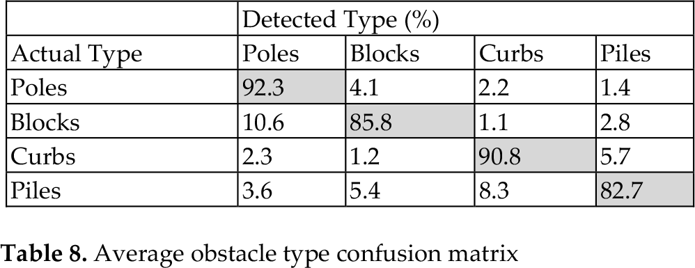
The confusion matrix shows that the major problem is how to distinguish bulky obstacles from thin ones. For example, “blocks” can be wrongly identified as “poles” (10.6%), and “piles” are incorrectly identified as “curbs” (8.3%). This is because, in urban scenes, one bulky obstacle may contain several isolated edges, resulting in several independent edge-blobs so that the bulky obstacle is split into several thin obstacles. The situation is similar when identifying thin obstacles from bulky ones. For example, when several pedestrians are very close to each other, their edge-blobs tend to merge into a single bulky one, which may result in an incorrect “block” identification. Despite the splitting and merging problems on edge-blobs, the distinguishing of vertical and planar types based on DRO features is more stable. For instance, “poles” are wrongly identified as “curbs” in only 2.2% of the cases, which shows the effect of the proposed DRO features in the top-view domain.

To test the verbal message generation scheme, a user walking trajectory is generated using the estimated safe direction and user's walking speed. This walking trajectory is then mapped to a top-view occupancy map generated using the obstacle detection algorithm. A segment of this synthesized map is shown in Figure 22, which is obtained from walking on an urban pedestrian pavement. The map is divided into 16 time slots: each slot corresponds to 5 seconds, which is the average time interval between delivered message sets. User's walking speed at each time slot is shown above the synthesized map, with estimated guidance state GS shown in the middle. The circles on the user's trajectory indicate the points where guidance messages are delivered. These points are indexed as 1 to 12 from left to right, and their corresponding message sets are listed in Table 9. It can be observed that hard-timing messages like safe directions are properly delivered at each transition point on the user trajectory. The fuzzy state estimator keeps track of the guidance state through each time slot. When the user enters a danger state with a high speed of 1.1 m/s, the system prompts “Please slow down” at point 1. When the user leaves the danger state and enters a normal state with a low speed of 0.8 m/s, the system prompts “You may walk faster” at point 4. These user motion messages are shown to be effective in adapting the user's walking speed according to different states.

Figure 22.

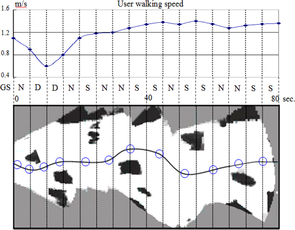
Simulation of user guidance

Table 9.

Delivered message sets.

Id	Message	Id	Message
1	Go 1 o'clock. Please slow down.	7	Go 12 o'clock. You may walk faster.
2	Go 12 o'clock.	8	Go 2 o'clock. Pile at 12 o'clock 10 steps.
3	Go 11 o'clock.	9	Go 12 o'clock. Pile at 10 o'clock 8 steps.
4	Go 12 o'clock. You may walk faster.	10	Pole at 1 o'clock 10 steps. Please slow down.
5	Pile at 10 o'clock 5 steps. Pole at 12 o'clock 14 steps.	11	Pole at 2 o'clock 3 steps. Pole at 10 o'clock 12 steps.
6	Go 11 o'clock. Pole at 12 o'clock 4 steps.	12	Block at 2 o'clock 13 steps. You may walk faster.

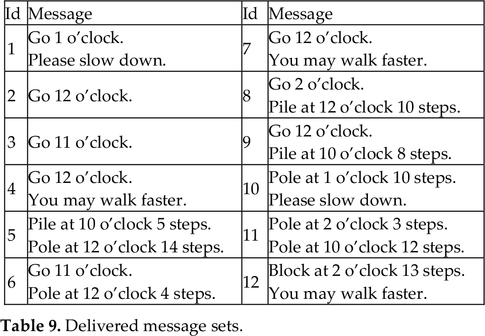
Soft-timing messages like those reporting obstacle positions follow the soft-timer, which is defined as: T₀ +τ·s. It can be observed that the message points are not evenly distributed between each five-second time slot. In a danger state when user speed is low, the message points are prompted densely, while in a safe state when user speed is high, the message points are prompted sparsely.

Under the experimental platform configuration shown in Table 5, the average runtime performance values of the major functions are listed in Table 10. If the system runs in full function mode, it can achieve an average frame rate of 12 fps on our experimental platform.

Table 10.

Runtime performance

Function	Ms/frame
Top-view mapping (with mapping table)	1.83
Edge-blob extraction and ellipse fitting	12.45
Obstacle type classification	1.26
Safe-area estimation and tracking	2.47
User motion estimation	61.32
Guidance state estimation	2.83
Total	82.16

In our experiment, a blind pedestrian walks at a speed of around 0.5 m/s∼1.8 m/s on average, a little bit slower than a normal pedestrian. At this walking speed, three to five seconds would be an appropriate time interval for message delivery, while a 2 fps image processing speed would be enough to meet the runtime requirement. Therefore, the proposed algorithm can fully satisfy the real-time requirements for a general outdoor guidance task.

To evaluate the system's real guidance performance, field tests with four visually impaired people are conducted. The characteristics of the four test subjects are listed in Table 11. All of the subjects use white canes as their usual mobility aids; the purpose of this field test is to evaluate whether the use of the proposed system will reduce the time required for the user to negotiate an unfamiliar pedestrian pavement.

Table 11.

Participants' characteristics for field test

ID	Gender	Age	Vision level	Usual aid
1	male	26	low	cane
2	male	31	none	cane
3	female	28	none	cane
4	female	30	low	cane

The field test areas are the same as the three test scenes shown in Figure 20 and Table 6. For each test scene, a test path 200 metres long is selected. The field test is carried out on the same day in the morning. The four test subjects are not familiar with the test paths selected. Before the real test starts, 30 minutes training is given to show the subjects how to use the system together with the white cane, and to explain the rules of the field test. In the field test, each subject is required to do two test runs on each path. For the first run, test subjects use both the guidance system and the white cane; for the second, they use only the white cane. In each test run, the time they take to pass along the 200-metre path is recorded. The data are presented in Figure 23.

Figure 23.

Walking time for each subject in field test

As shown in Figure 23a, on the open-space path, the average time for the first run is 154 seconds, and for second run 185 seconds. The guidance system therefore improves the user's travelling speed by 17%. On the urban path, with narrower space and more obstacles, the use of the guidance system in the first run brings an even bigger improvement of 28.5% in the user's average travelling speed. The results show that our system leads to a reduction of almost 30% in the time taken to negotiate obstacles after only a few minutes training with the system.

On the urban test path, some low piles built to prevent illegal parking represented a very high threat for blind pedestrians using only the white cane. These situations are shown in Figure 24. In the second run on the urban path, the subjects equipped only with the white cane did spot the danger presented by these low piles. However, in the first run with the guidance system, these low piles could be detected much further ahead of the user, and verbal feedback given to help keep them away from those potential collision threats.

Figure 24.

Low piles on urban path

After the field test, the test subjects all agreed that the system was capable of detecting and identifying obstacles effectively within a medium range, providing intuitive verbal feedback at appropriate times that was easy to interpret and act upon. A few limitations of the proposed system were also observed. The first limitation is the assumption of a flat road plane. The second is that the camera is required to be fixed on the user's body at a certain downward viewing angle, and camera parameters are required for top-view mapping.

6. Conclusion

This paper has presented a mono-vision-based guidance system for blind people in an outdoor environment. Its first contribution is in presenting an effective way to discriminate obstacles from a cluttered background by means of inhomogeneous top-view re-sampling. It has also presented the directional ellipse model and DRO feature in the top-view domain for obstacle type classification. For guidance, polar histogram tracking can make safe-area estimation more reliable; meanwhile, a fuzzy state estimator can provide valuable state information for message delivery. Our real field tests show that the described techniques allow the system to be usefully applied in real-time obstacle detection and guidance on complex-scene pedestrian pathways.