Sage Journals: Discover world-class research

Abstract

The development of accurate control systems for underwater robotic vehicles relies on the adequate compensation of thruster dynamics. Without compensation, the closed-loop positioning system can exhibit limit cycles. This undesired behaviour may compromise the overall system stability. In this work, a fuzzy sliding-mode compensation scheme is proposed for electrically actuated bladed thrusters, which are commonly employed in the dynamic positioning of underwater vehicles. The boundedness and convergence properties of the tracking error are analytically proven. The numerical results suggest that this approach shows a greatly improved performance when compared with an uncompensated counterpart.

Keywords

Fuzzy Logic Sliding-Modes Thruster Dynamics Underwater Robotic Vehicles

1. Introduction

The dynamic behaviour of a remotely operated underwater vehicle (ROV) can be greatly influenced by the nonlinear dynamics of the vehicle thrusters. In this way, the implementation of a proper control strategy for the thruster subsystem is essential for the accurate control of the entire robotic vehicle.

A growing number of papers dedicated to the dynamic positioning of ROVs confirms the necessity of the development of a controller, that could deal with the inherent nonlinear system dynamics, imprecise hydrodynamic coefficients, and external disturbances [4]. Many of these works [12, 25 –27] address the problem of the influence of thruster dynamics on overall vehicle behaviour, and the importance of considering this effect in the dynamic positioning system.

Traditionally, some mathematical models of the thruster are used directly to estimate, in a feed-forward manner, the required voltage (or current) to produce the desired thrust force. This strategy has simplicity as an advantage and the fact that it does not require the angular velocity of the propeller to be measured. On the other hand, it can only be used with a precise mathematical model of the thruster system. The adoption of a standard model, available in the literature but not perfectly suited to the actual thrusters, is in many situations the reason for the poor tracking performance of a ROV. It has been previously reported [27], that this approach can lead to limit cycles in the closed-loop positioning system. As also shown in [27], this degradation in the controller performance is specially critical during low-speed manoeuvres with the vehicle. In such cases, the dynamic behaviour of underwater robotic vehicles can be dominated by thruster dynamics.

An alternative approach that may be considered, specially when a precise mathematical model for the thruster system cannot be obtained, is the design of a feedback compensation scheme for thruster dynamics. In this work, a sliding-mode compensator with fuzzy gain is proposed to calculate the required voltage for each thruster. The choice of a variable gain, defined by a fuzzy inference system, makes a better trade-off between reaching time and tracking precision possible. The adoption of a saturation function (instead of a relay function) within the control law leads to a boundary layer, that can minimize or, when desired, even completely eliminate chattering. Through a Lyapunov-like analysis, the boundedness and convergence properties of the closed-loop compensation subsystem is proven. Numerical simulations are carried out to demonstrate the robustness and improved performance of the compensation strategy.

2. Vehicle Dynamics Model

An adequate model to describe the dynamic behaviour of an underwater robotic vehicle must include the rigid-body dynamics of the vehicle and a representation of the surrounding fluid dynamics. In this context, the ideal mathematical model would be composed of a system of ordinary differential equations, to represent rigid-body dynamics, and partial differential equations to represent fluid dynamics.

In order to overcome the computational problem of solving a system with this degree of complexity, in the majority of publications [1, 3, 4, 7, 13 –16, 23, 28] a lumped-parameters approach is employed to approximate the vehicle's dynamic behaviour.

The equations of motion for underwater vehicles can be presented with respect to an inertial reference frame or with respect to a body-fixed reference frame, Fig. 1. On this basis, the equations of motion for underwater vehicles can be expressed, with respect to the body-fixed reference frame, in the following vectorial form:

Figure 1.

Underwater vehicle with both inertial and body-fixed reference frames.

M \dot{ν} + k (ν) z d v h (ν) + g (x) = τ

(1)

where ν = [ν_x, ν_y, _z ,ω_x,ω_y, ω_z] is the vector of linear and angular velocities in the body-fixed reference frame, x = [x, y, z, α, β, γ] represents the position and orientation with respect to the inertial reference frame, M is the inertia matrix, which accounts not only for the rigid-body inertia but also for the so-called hydrodynamic added inertia, k(ν) is the vector of generalized Coriolis and centrifugal forces, h(ν) represents the hydrodynamic quadratic damping, g(x) is the vector of generalized restoring forces (gravity and buoyancy) and τ is the vector of control forces and moments.

It should be noted that in the case of remotely operated underwater vehicles (ROVs), the metacentric height is sufficiently large to provide the self-stabilization of roll (α) and pitch (β) angles. This particular constructive aspect also allows the order of the dynamic model to be reduced to four degrees of freedom, x = [x, y, z, γ], and the vertical motion (heave) to be decoupled from the motion in the horizontal plane. This simplification can be found in the majority of works presented in the literature [4, 8, 11, 13 –15, 19, 28, 29]. Thus, the positioning system of a ROV can be divided in two different parts: depth control (concerning variable z), and control in the horizontal plane (variables x, y and γ).

In this context, considering that control forces and moments are produced by the thrusters of the vehicle, the dynamic model of the thruster subsystem is discussed in the following subsection.

2.1. Dynamic Thruster Model

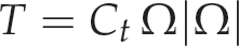
The steady-state axial thrust (T) produced by marine thrusters is commonly presented as proportional to the square of the angular velocity Ω of the propeller [18]. This quadratic relationship can be conveniently represented by

T = C_{t} Ω | Ω |

(2)

where C_t is a function of the advance ratio and depends on the constructive characteristics of each thruster.

Taking the dynamical behaviour of the thruster system into account, Yoerger et al. [27] presented a first order nonlinear dynamic thruster model with propeller angular velocity as the state variable. This dynamic model, that can be represented by Eq. (3) and Eq. (4), is referred to here as Model 1.

J_{m s p} \dot{Ω} + K_{v} Ω | Ω | = Q_{m}

(3)

T = C_{t} Ω | Ω |

(4)

where J_msp is the motor-shaft-propeller inertia, K_v stays for a model parameter, and Q_m is the input motor torque.

In later works [2, 10, 12], more accurate models employing lift and drag curves, and that also incorporate some other hydrodynamic effects, such as those caused by the rotational fluid velocity, are proposed. In all of these models, a second order dynamic system with propeller angular velocity and axial fluid velocity as state variables is used. However, during real operations with an underwater robotic vehicle, the axial fluid velocity cannot be measured with the required precision, which compromises its application for control purposes as a model state variable.

Nevertheless, if the following physically justified assumptions could be made:

Magnitude and direction of axial fluid velocity are mainly determined by the propeller's rotational velocity,

Interference of the flow from one thruster to another is negligible,

Ambient fluid velocity and the ROV's manoeuvring speed are negligible, when compared with the axial fluid velocity generated by the propeller's rotation,

the simplified first order dynamic model proposed by Yoerger et al. [27], Model 1, can satisfactorily be used as a part of the compensation strategy in thrust control. The use of only propeller angular velocity (Ω) as a state variable is advantageous because it can easily be measured (or estimated) during real-time operations with a sensor coupled to the motor's shaft.

However, considering recent experimental results, marine thrusters may also exhibit non-smooth nonlinearities such as dead-zones. A dead-zone is a hard nonlinearity, frequently encountered in many industrial actuators, and its presence can drastically reduce control system performance and lead to limit cycles in a closed-loop system. The experiments were carried out in a wave channel with the thruster units of a small remotely operated underwater vehicle, developed at the Institute of Mechanics and Ocean Engineering of the Hamburg University of Technology. The ROV is equipped with eight thrusters for dynamic positioning and a passive arm for position and attitude measurement. A picture of the experimental underwater vehicle is presented in Fig. 2.

Figure 2.

The experimental remotely operated underwater vehicle.

Therefore, taking the experimental data into account, we propose a variation of Model 1 by incorporating some limitations of the actuator. This modified version, identified here as Model 2, can be mathematically represented by equations (5)–(6):

J_{m s p} \dot{Ω} + K_{v 1} Ω + K_{v 2} Ω | Ω | = \frac{K_{t}}{R_{m}} V_{m}

(5)

T = D (Ω | Ω |)

(6)

where V_m is the input voltage and D(Ω|Ω|) represents a dead-zone nonlinearity with a quadratic input Ω|Ω| and output T, which can be mathematically described by:

D (Ω | Ω |) = {\begin{array}{l} K_{l} (Ω | Ω | - δ_{l}) & for Ω | Ω | \leq δ_{l} \\ 0 & for δ_{l} < Ω | Ω | < δ_{r} \\ K_{r} (Ω | Ω | - δ_{r}) & for Ω | Ω | \geq δ_{r} \end{array}

The constants K_t and R_m, which represent the motor torque constant and winding resistance, respectively, can be obtained from the data-sheet. The values of K_v1, K_v2, K_l, K_r, δ_l and δ_r depend on the constructive characteristics of each thruster and must be experimentally determined. For control purposes, these parameters are treated here as constants for each thruster unit. This simplification is acceptable, as shown in the next section, due to the robustness of the proposed controller to parametric uncertainties.

By incorporating the term K_v1Ω in Eq. (5), Model 2 takes the back electromotive force and the viscous damping, due to mechanical sealing, into account. The term K_v2Ω|Ω| represents the propeller rotational torque due to hydrodynamic loading. By adopting Eq. (6) to describe the relationship between the propeller's angular velocity and thrust force, the modified model also considers friction losses during the propeller's rotation. In the majority of works, the effect of friction losses is neglected.

The experimental data obtained in a wave channel with the thruster unit of the ROV can be used to validate the proposed modifications to Model 1. Figure 3 shows a comparative analysis between Model 1 [27], Model 2 (modified model) and the experimental thruster's response. The required parameters for both models are obtained using the Levenberg–Marquadt algorithm [17].

Figure 3.

Comparative analysis between Model 1, Model 2 and the experimental data.

As observed in Fig. (3), Model 2 is better suited than Model 1 to representing the response of the thruster unit. This improvement is due to the incorporation of some of the thruster's electro-mechanical characteristics and the effect of friction losses during the propeller's rotation in the model. Such effects, that probably may be neglected in optimized thrusters, must be considered with the application of low-cost units.

3. Dynamic Positioning System

The dynamic positioning of underwater robotic vehicles is essentially a multivariable control problem. Nevertheless, as demonstrated by Slotine [21], the variable structure control methodology allows different controllers to be separately designed for each degree of freedom (DOF).

Over the past decades, decentralized control strategies have been successfully applied to the dynamic positioning of underwater vehicles [6, 8, 15, 20, 23, 28].

Considering that the control law for each degree of freedom can be easily designed with respect to the inertial reference frame, Eq. (1) should be rewritten in this coordinate system.

Remembering that

\dot{x} = J (x) ν

(7)

where J(x) is the Jacobian transformation matrix, it can be directly implied that

ν = J^{- 1} (x) \dot{x}

(8)

and

\dot{ν} = {\dot{J}}^{- 1} \dot{x} + J^{- 1} \ddot{x}

(9)

Therefore, the equations of motion of an underwater vehicle, with respect to the inertial reference frame, becomes

\bar{M} \ddot{x} + \bar{k} + \bar{h} = \bar{τ}

(10)

where $\bar{M} = J^{- T} M J^{- 1}$ , $\bar{k} = J^{- T} k + J^{- T} M {\dot{J}}^{- 1} \dot{x}$ , $\bar{h} = J^{- T} h$ and $\bar{τ} = J^{- T} τ$ .

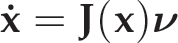
In order to develop the control law with a decentralized approach, Eq. (10) can be rewritten as follows:

{\ddot{x}}_{i} = {\bar{m}}_{i}^{- 1} ({\bar{τ}}_{i} - {\bar{k}}_{i} - {\bar{h}}_{i}); i = 1,2,3,4,

(11)

where $x_{i}$ , ${\bar{τ}}_{i}$ , ${\bar{k}}_{i}$ and ${\bar{h}}_{i}$ are the components of $x = [x, y, z, γ]$ , $\bar{τ}$ , $\bar{k}$ and $\bar{h}$ , respectively. Concerning ${\bar{m}}_{i}$ , it represents the main diagonal terms of J^−TMJ⁻¹.

For notational simplicity the index i will be suppressed in Eq. (11) and, in this way, the equation of motion for each degree of freedom (DOF) becomes:

\ddot{x} = {\bar{m}}^{- 1} (\bar{τ} - \bar{k} - \bar{h})

(12)

In order to facilitate the analysis of the influence of thruster dynamics on the overall system behaviour, a 1-DOF underwater vehicle model with exactly known parameters is considered here. Otherwise, the actual effect of thruster dynamics over the vehicle dynamics would be masked by some variable parameters and cross-coupling effects.

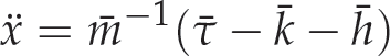
Therefore, based on the assumption of well-known parameters and to highlight the influence of thruster dynamics, a feedback linearization approach is adopted for the dynamic positioning of the underwater robotic vehicle. The proposed control law can be written as

\bar{τ} = \bar{k} + \bar{h} + \bar{m} ({\ddot{x}}_{d} - 2 λ \dot{\tilde{x}} - λ^{2} \tilde{x})

(13)

where x_d is the desired trajectory, $\tilde{x} = x - x_{d}$ is the tracking error and λ is a positive constant.

For this closed-loop system, composed by Eq. (12)–(13), we have the following error dynamics:

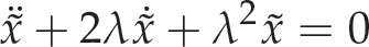
\ddot{\tilde{x}} + 2 λ \dot{\tilde{x}} + λ^{2} \tilde{x} = 0

(14)

with coefficients that satisfy a Hurwitz polynomial and ensure exponential convergence to zero.

Now, considering the required thrust to make the vehicle follow a prescribed trajectory, defined by Eq. 13, we can calculate the desired force that should be produced by each thruster by T_d = τ/N_T, where N_T is the available number of thrusters to actuate within the desired direction.

Finally, considering Eq. (6), a dead-zone inverse is used to compute the desired propeller angular velocity Ω_d. It should be highlighted that, in order to define the dead-zone inverse, parameters K_l, K_r, δ_l and δ_r must be exactly known. If these parameters are uncertain or could not be experimentally obtained, a robust dynamic positioning system [3, 4] or a dead-zone compensation scheme [5] should be taken into account.

3.1. Thruster Dynamics Compensation

In order to develop the compensation scheme, Eq. (5) can be rewritten as follows:

a \dot{Ω} + b Ω + c Ω | Ω | = u

(15)

where u is the input voltage and a, b and c are variable but positive and bounded parameters. If these parameters were perfectly known, then the following compensator would be enough to deal with the thruster's dynamic:

u = b Ω + c Ω | Ω | + a {\dot{Ω}}_{d}

(16)

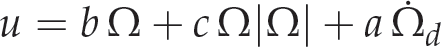
Considering that only the estimates â, $\hat{b}$ and ĉ are available, let the compensation problem be treated in Filippov's way [9], defining a law composed by an equivalent control $\hat{u} = \hat{b} Ω + \hat{c} Ω | Ω | + \hat{a} {\dot{Ω}}_{d}$ and a discontinuous term −𝒦sgn(s):

u = \hat{b} Ω + \hat{c} Ω | Ω | + \hat{a} {\dot{Ω}}_{d} - K sgn (s)

(17)

where $s = \tilde{Ω} = Ω - Ω_{d}$ , Ω_d is the desired propeller angular velocity, 𝒦 is the compensator gain (which in this work is variable and determined by a fuzzy inference system), and sgn(·) is defined by

sgn (s) = {\begin{array}{r} - 1 & if s < 0 \\ 0 & if s = 0 \\ 1 & if s > 0 \end{array}

Regarding the development of the control law, the following assumption must be made:

Assumption 1. The desired propeller angular acceleration ( ${\dot{Ω}}_{d}$ ) is continuous, available and with known bounds.

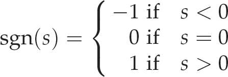
In this work, the desired propeller angular acceleration ( ${\dot{Ω}}_{d}$ ) is estimated using the backward difference method.

The compensator established in Eq. (17) is based on the classical sliding-mode control that originally appeared in Soviet literature [24]. It is able to deal with the parametric uncertainties but, as a drawback, leads to high control activity and chattering. To overcome these limitations, the relay function sgn(·) in Eq. (17) can be replaced by a saturation function [22], defined as:

sat (s / ϕ) = {\begin{matrix} sgn (s) & if | s / ϕ | \geq 1 \\ s / ϕ & if | s / ϕ | < 1 \end{matrix}

The substitution of sgn(·) by sat(·) leads to the appearance of a boundary layer (Φ) with width ϕ, which turn perfect tracking into a tracking with guaranteed precision problem.

In order to demonstrate that the proposed compensation scheme can deal with unstructured uncertainties, the term bΩ is treated as unmodelled dynamics and not taken into account within the design of the control law:

u = \hat{c} Ω | Ω | + \hat{a} {\dot{Ω}}_{d} - K sat (\frac{s}{ϕ})

(18)

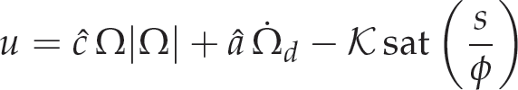
Figure 4 shows the block diagram of the resulting dynamic positioning system.

Figure 4.

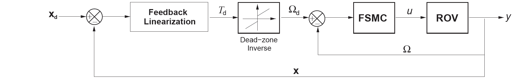
Block diagram of the ROV controller with fuzzy sliding-mode compensation for thruster dynamics.

On this basis, a variable gain, defined by a fuzzy inference system, is chosen in order to make a better trade-off between reaching time and tracking precision. The adopted fuzzy inference system is the zero order TSK (Takagi–Sugeno–Kang), whose rules can be stated in a linguistic manner as follows:

\begin{array}{l} I f | s | i s S_{n} t h e n k_{n} = k_{n} & ; & n = 1, 2 \dots, N \end{array}

where S_n are fuzzy sets, and K_n is the output value of each one of the N fuzzy rules, with K_n > K_n–1. Triangular (in the middle) and trapezoidal (at the edges) membership functions could, for instance, be adopted for the fuzzy sets.

Considering that each rule defines a numerical value as output K_n, the final output 𝒦 can be computed by a weighted average:

K = \frac{\sum_{n = 1}^{N} w_{n} \cdot k_{n}}{\sum_{n = 1}^{N} w_{n}}

(19)

where w_n is the firing strength of each rule.

According to Lemma 1, Eq. (19) implies that 𝒦 is bounded.

Lemma 1. Let the fuzzy gain 𝒦 be defined by Eq. (19), then 𝒦 is bounded, K_min ≤ 𝒦 ≤ K_max.

Proof. Equation (19) may also be written as 𝒦 = K^TΨ(s), where K = [K₁, K₂,…, K_N] is the vector containing attributed values to each rule, with K_n > K_n–1, and $Ψ (s) = [ψ_{1} (s), ψ_{2} (s), \dots, ψ_{N} (s)]$ is a vector with components $ψ_{n} (s) = w_{n} / \sum_{n = 1}^{N} w_{n}$ . So, for the adopted membership functions (triangular in the middle and trapezoidal at the edges), with the central values chosen as: C = {C₁; C₂; …; C_N}, we have for s ≤ C₁, Φ (s) = [1, 0,…, 0, 0], which implies K = K₁. In the same way, for s ≥ C_N we have Φ(s) = [0, 0,…, 0, 1], which implies 𝒦 = K_N, and completes the proof: K₁ ≤ 𝒦 ≤ K_N.▪

The boundedness and convergence properties of the proposed compensation scheme relies on the following theorem.

Theorem 1. For the thruster system represented by Eq. (15), the fuzzy sliding-mode compensator defined by Eq. (18) and Eq. (19), with $K_{1} = F + \hat{a} α η + \hat{a} (α - 1) | {\dot{Ω}}_{d} |$ , ensures the boundedness of all closed-loop signals and the finite time convergence to $Φ = {Ω | | \tilde{Ω} | \leq ϕ}$ .

Proof. To establish boundedness of the closed-loop signals, let us first define a Lyapunov function candidate V, where

V (t) = \frac{1}{2} s_{ϕ}^{2}

(20)

and sϕ is a measure of the distance of the current state to the boundary layer (Φ), that can be defined as

s_{ϕ} = s - ϕ sat (s / ϕ)

(21)

Noting that sϕ = 0 inside the boundary layer and ${\dot{s}}_{ϕ} = \dot{s}$ , we have $\dot{V} (t) = 0$ inside Φ, and outside:

\dot{V} (t) = s_{ϕ} {\dot{s}}_{ϕ} = s_{ϕ} \dot{s} = (\dot{Ω} - {\dot{Ω}}_{d}) s_{ϕ} = [a^{- 1} (f + u) - {\dot{Ω}}_{d}] s_{ϕ}

where $u = - \hat{f} + \hat{a} {\dot{Ω}}_{d} - K sgn (s)$ outside the boundary layer, $f = - b Ω - c Ω | Ω |$ and $\hat{f} = - \hat{c} Ω | Ω |$ . So, the time derivative of s takes the following form:

\dot{s} = a^{- 1} [f - \hat{f} + \hat{a} \dot{Ω} - K sgn (s)] - {\dot{Ω}}_{d}

(22)

If the parameters a, b and c are unknown but assumed to be positive and bounded, which is physically coherent, and their estimates â and ĉ are both positive constants, so that $| \hat{f} - f | \leq F$ and α⁻¹ ≤ â/a ≤ α, where $α = \sqrt{a_{m a x} / a_{m i n}},$ then we have:

\dot{V} (t) = [a^{- 1} (f + u) - {\dot{Ω}}_{d}] s_{ϕ}

(23)

= {a^{- 1} [f - \hat{f} + \hat{a} {\dot{Ω}}_{d} - K sgn (s)] - {\dot{Ω}}_{d}} s_{ϕ}

(24)

= - [a^{- 1} (\hat{f} - f) + {\dot{Ω}}_{d} - a^{- 1} \hat{a} {\dot{Ω}}_{d} + a^{- 1} K sgn (s)] s_{ϕ}

(25)

>From Lemma 1, defining $K_{m i n} = F + \hat{a} α η + \hat{a} (α - 1) | {\dot{Ω}}_{d} |$ , with η being a positive constant related to the convergence time, implies that 𝒦 ≥ K_min and that

\dot{V} (t) \leq - η | s_{ϕ} |

(26)

implying that V(t) ≥ V(0), and, therefore, that sϕ is bounded. From the definition of sϕ, Eq. (21), we can conclude that s is also bounded. Considering Eq. (22), Lemma 1 and Assumption 1, it can be easily verified that $\dot{s}$ is also bounded.

Integrating both sides of (26) between 0 and t_reach, where sϕ(t_reach) = 0, shows that $Φ = {Ω | | \tilde{Ω} | \leq ϕ}$ will be reached in a finite time smaller than

t_{reach} \leq \frac{| s_{ϕ} (t = 0) |}{η}

(27)

This ensures the finite time convergence to the boundary layer and the boundedness of the closed-loop signals, completing the proof.▪

Theorem 1 also implies that the boundary layer is an invariant set, i.e., every system trajectory which starts from a point in Φ remains in Φ for ∀t ≥ 0. Inside the boundary layer Φ, the error dynamics takes the following form:

a \dot{s} + \frac{K}{ϕ} s = p^{T} y

(28)

where $p = [(\hat{a} - a), - b, (\hat{c} - c)]$ is the vector with parametric uncertainty, and $y = [{\dot{Ω}}_{d}, Ω, Ω | Ω |]$ .

4. Simulation Results

The simulation studies were performed with a numerical implementation in C, with sampling rates of 500 Hz for ROV states and 1 kHz for propeller rotational velocity. The chosen parameters for the thruster model are: k_r = k_l = 2.25×10⁴, δ_r = −δ_l = 5.75 × 10⁻⁵, a(t) = 1.0 × 10⁻² · ∊(t), b(t) = 4.0 × 10⁻² · ∊(t) and c(t) = 1.4 × 10⁻⁵ · ∊(t), with ∊(t) = 1 + 0.25 sen (|Ω|t). The ROV model is defined with $\bar{m} = 50$ kg, $\bar{k} = 0$ , $\bar{h} = 0.5 ρ C_{D} A \dot{x} | \dot{x} |$ , A = 0.25 m², ρ = 1000 kg/m³ and C_D = 1.2.

The performance of the proposed compensator, Eq. (18), is evaluated first in comparison with a conventional sliding-mode compensator. The chosen parameters for the FSMC are â = 1.0 × 10⁻², ĉ = 1.1 × 10⁻⁴ and ϕ = 7.0. For the fuzzy gain (K), triangular (in the middle) and trapezoidal (at the edges) membership functions are adopted for S_n, with the central values defined as C = {7.0; 15.0; 25.0; 50.0; 100.0; 200.0; 400.0} and associated crisp outputs K_n = {1.0; 1.5; 2.0; 3.0; 4.0; 6.0; 10.0} × K_min, where $K_{m i n} = F + \hat{a} α η + \hat{a} (α - 1) | {\dot{Ω}}_{d} |$ , F = 6.8, α = 1.29 and η = 0.15. For the conventional sliding-mode controller we set K as constant, K = K_min. Figure 5 shows some comparative results between FSMC and SMC.

Figure 5.

Propeller's angular velocity (top) and the related input voltage (bottom) for both the fuzzy sliding-mode compensator (FSMC) and the conventional sliding-mode compensator (SMC).

Figure 5 shows that the fuzzy sliding-mode compensator (FSMC) is capable of providing the stabilization of the desired propeller angular velocity even in the presence of both structured and unstructured uncertainties. It could also be observed that the FSMC shows a better and almost constant rising time for different values of Ω_d, without increasing control activity and chattering.

Now, in order to demonstrate the improved performance of the dynamic positioning system with the FSMC over the commonly adopted feed-forward approach, we show a comparison of both strategies for two different trajectories: x_d = 0.05[1 – cos(0.25πt)] (Fig. 6) and x_d = 0.25[1 – cos(0.5πt)] (Fig. 7). In both cases, the input voltage in the feed-forward approach was directly estimated, based on thruster Model 2, with $u = \hat{b} Ω_{d} + \hat{c} Ω_{d} | Ω_{d} |$ , with $\hat{b} = 4.0 \times 10^{- 2}$ and ĉ = 1.4 × 10⁻⁵.

Figure 6.

Comparative analysis of the ROV positioning system with the proposed FSMC and with a feed-forward approach based on Model 2 (M2BC) for the tracking of x_d = 0.05[1 – cos(0.25πt)] m.

Note that despite the better suited parameters of the feed-forward approach (M2BC), the proposed compensation scheme (FSMC) shows an improved performance. This is due to the ability of the FSMC to track the necessary angular velocity for the propeller, Fig. 6(c) and Fig. 7(c). Comparing Fig. 6(b) with Fig. 7(b), it could also be verified that the degradation in the controller performance, caused by the influence of thruster dynamics, is specially critical during low-speed manoeuvres with the vehicle. This result confirms that, in such cases, the dynamic behaviour of an underwater robotic vehicle can be dominated by thruster dynamics.

Figure 7.

Comparative analysis of the ROV positioning system with the proposed FSMC and with a feed-forward approach based on Model 2 (M2BC) for the tracking of x_d = 0.25[1 – cos(0.5πt)] m.

5. Concluding Remarks

The present work addresses the compensation of thruster dynamics in the dynamic positioning system of underwater robotic vehicles. A sliding-mode compensator with fuzzy gain is proposed to enhance the tracking performance. The boundedness of the closed-loop signals' compensation subsystem, as well as the finite time convergence of the error to the boundary layer, is proven using Lyapunov's stability theory. By means of numerical simulations, the improved performance and the robustness to both structured and unstructured uncertainties, namely parametric uncertainties and unmodelled dynamics, are confirmed.

Footnotes

6. Acknowledgements

The authors would like to acknowledge the support of the Brazilian National Research Council (CNPq), the Brazilian Coordination for the Improvement of Higher Education Personnel (CAPES) and the German Academic Exchange Service (DAAD).

References

Antonelli

[2007]. On the use of adaptive/integral actions for six-degrees-of-freedom control of autonomous underwater vehicles, IEEE Journal of Oceanic Engineering 32(2): 300–312.

Bachmayer

Whitcomb

L. L.

[2003]. Adaptive parameter identification of an accurate nonlinear dynamical model for marine thrusters, ASME Journal of Dynamic Systems, Measurement, and Control 125(3): 491–494.

Bessa

W. M.

Dutra

M. S.

Kreuzer

[2008]. Depth control of remotely operated underwater vehicles using an adaptive fuzzy sliding-mode controller, Robotics and Autonomous Systems 56(8): 670–677.

Bessa

W. M.

Dutra

M. S.

Kreuzer

[2010]. An adaptive fuzzy sliding-mode controller for remotely operated underwater vehicles, Robotics and Autonomous Systems 58(1): 16–26.

Bessa

W. M.

Kreuzer

[2011]. sliding-mode control of a remotely operated underwater vehicle with adaptive fuzzy dead-zone compensation, Proceedings in Applied Mathematics and Mechanics 11(1): 803–804.

Chatchanayuenyong

Parnichkun

[2007]. Neural network based-time optimal sliding-mode control for an autonomous underwater robot, Mechatronics 16: 471–478.

Corradini

M. L.

Monteriù

Orlando

[2011]. An actuator failure tolerant control scheme for an underwater remotely operated vehicle, IEEE Transactions on Control Systems Technology 19(5): 1036–1046.

Da Cunha

J. P. V. S.

Costa

R. R.

Hsu

[1995]. Design of a high performance variable structure control of ROVs, IEEE Journal of Oceanic Engineering 20(1): 42–55.

Filippov

A. F.

[1988]. Differential Equations with Discontinuous Right-hand Sides, Kluwer, Dordrecht.

10.

Fossen

T. I.

Blanke

[1994]. Nonlinear output feedback control of underwater vehicle propellere using feedback from estimated axial flow velocity, IEEE Journal of Oceanic Engineering 25(2): 241–255.

11.

Guo

Chiu

F. C.

Huang

C. C.

[2003]. Design of a sliding-mode fuzzy controller for the guidance and control of an autonomous underwater vehicle, Ocean Engineering 30: 2137–2155.

12.

Healey

A. J.

Rock

S. M.

Cody

Miles

Brown

J. P.

[1995]. Toward and improved understanding of thruster dynamics for underwater vehicles, IEEE Journal of Oceanic Engineering 20(4): 354–361.

13.

Hoang

N. Q.

Kreuzer

[2007]. Adaptive PD-controller for positioning of a remotely operated vehicle close to an underwater structure: theory and experiments, Control Engineering Practice 15: 411–419.

14.

Hsu

Costa

R. R.

Lizarralde

Da Cunha

J. P. V. S.

[2000]. Dynamic positioning of remotely operated underwater vehicles, IEEE Robotics and Automation Magazine 7(3): 21–31.

15.

Kiriazov

Kreuzer

Pinto

F. C.

[1997]. Robust feedback stabilization of underwater robotic vehicles, Robotics and Autonomous Systems 21: 415–423.

16.

Yang

Ding

Bogdan

[2012]. Robust adaptive motion control for underwater remotely operated vehicles with velocity constraints, International Journal of Control, Automation, and Systems 10(2): 421–429.

17.

Marquardt

D. W.

[1963]. An algorithm for least squares estimation of nonlinear parameters, SIAM Journal of the Society of Industrial and Applied Mathematics 11: 431–441.

18.

Newman

J. N.

[1986]. Marine Hydrodynamics, 5th edn, MIT Press, Massachusetts.

19.

Pinto

F. C.

[1996]. Theoretische und experimentelle Untersuchung zur Sensorik und Regelung von Unterwasserfahrzeugen, VDI Verlag, Düsseldorf.

20.

Sebastiãαn

Sotelo

M. A.

[2007]. Adaptive fuzzy sliding-mode controller for the kinematic variables of an underwater vehicle, Journal of Intelligent and Robotic Systems 49: 189–215.

21.

Slotine

J.-J. E.

[1983]. Tracking Control of Nonlinear Systems Using Sliding Surfaces, Tese (Ph.D.), Massachusetts Institute of Technology, Cambridge.

22.

Slotine

J.-J. E.

[1991]. Applied Nonlinear Control, Prentice Hall, New Jersey.

23.

Smallwood

D. A.

Whitcomb

L. L.

[2004]. Model-based dynamic positioning of underwater robotic vehicles: Theory and experiment, IEEE Journal of Oceanic Engineering 29(1): 169–186.

24.

Utkin

V. I.

[1978]. Sliding-modes and Their Application to Variable Structure Systems, MIR Publishers, Moscow.

25.

Whitcomb

L. L.

Yoerger

D. R.

[1999a]. Development, comparison, and preliminary experimental validation of non-linear dynamic thruster models, IEEE Journal of Oceanic Engineering 24(4): 481–494.

26.

Whitcomb

L. L.

Yoerger

D. R.

[1999b]. Preliminary experiments in model-based thruster control for underwater vehicle positioning, IEEE Journal of Oceanic Engineering 24(4): 495–506.

27.

Yoerger

D. R.

Cooke

J. G.

Slotine

J.-J. E.

[1990]. The influence of thruster dynamics on underwater vehicle behavior and their incorporation into control system design, IEEE Journal of Oceanic Engineering 15(3): 167–178.

28.

Yoerger

D. R.

Slotine

J.-J. E.

[1985]. Robust trajectory control of underwater vehicles, IEEE Journal of Oceanic Engineering 10(4): 462–470.

29.

Zanoli

S. M.

Conte

[2003]. Remotely operated vehicle depth control, Control Engineering Practice 11: 453–459.

Dynamic Positioning of Underwater Robotic Vehicles with Thruster Dynamics Compensation

Abstract

Keywords

1. Introduction

2. Vehicle Dynamics Model

Footnotes

6. Acknowledgements

References