Sage Journals: Discover world-class research

Abstract

The Path-Planning problem is a basic issue in mobile robotics, in order to allow the robots to solve more complex tasks, for example, an exploration assignment in which the distance given by the planner is taken as a utility measure. Among the different proposed approaches, algorithms based on an exact cell decomposition of the environment are very popular. In this paper, we present a new algorithm for universal path planning in cell decomposition, using a raster scan method for computing the Exact Euclidean Distance Transform (EEDT) for each cell in the map. Our algorithm computes, for every cell in the map, the point sequence to the goal. For each sequence, the sub-goals are selected near to the vertices of the obstacles, reducing the total distance to the goal without post processing. At the end, we obtain a smooth path up to the goal without the need for post-processing. The paths are computed by visibility verification among the cells, exploiting the processing performed in the neighbouring cells.

Keywords

Path Planning Cell Decomposition Distance Transform

1. Introduction

The path-planning problem is a fundamental challenge in mobile robotics. Applications include search and rescue, hazardous material handling, planetary exploration, etc. A specific application of path planning is exploration and mapping [1 –3], where the planner is responsible for efficiently reaching the given objectives. The distance given by the planner to each goal is taken as a utility measure in some exploration algorithms; therefore it is necessary to have an algorithm that provides accurate distances towards the goal.

A good technique for path planning is the approach based on visibility graphs, which contain the start vertex, the goal vertex and the corners of all blocked cells [4]. A vertex is connected via a straight line to another vertex if there is a line-of-sight between the vertices, that is, the straight line does not pass through a blocked cell. The shortest paths on visibility graphs are also the shortest paths in the full environment. However, solving a path-planning problem with visibility graphs can be slow when considering complex environments.

The global path-planning problem can be defined as follows: Given a robot and the description of an environment, to plan a collision-free continuous path between two specified locations for the robot, while a certain optimization criterion is satisfied [5]. Such a problem is PSPACE-Complete in general and for some cases is NP-Complete [6].

The classical methods for global path planning are variations of a few general approaches: roadmaps, cell decomposition, artificial potential fields and mathematical programming [7].

The problem of universal path planning can be defined as follows: Planning is the goal-directed selection of reactions to all possible situations [8,9].

The principle of exact cell decomposition is to divide the environment C of the robots in a collection of non-overlapping regions, called cells [10], so each cell of the grid is marked as free or occupied.

The Distance Transform algorithms (also called wave front or bushfire methods) are propagation algorithms widely used in exact cell decomposition path planning. In this paper we address the problem of path planning based on an exact cell decomposition of the environment, obtaining a good distance transform from all cells towards the goal and identifying the best sequence of sub-goals up to the target. The path generated by our approach for each cell is similar to the path obtained using the visibility graph approach. A short version of this paper has been already published in [11]; here, we add extra tests and perform further analysis of the results.

This paper is organized as follows: Section 2 expounds previous work and explains the principle of distance transform algorithms. Section 3 outlines our approach to the path-planning problem and Section 4 presents numerical results that show the performance of our method. In Section 5 we present our conclusions and discussions for future research.

2. Related Work

The most popular algorithms for solving path-planning problems using cell decomposition of the environment are the A^* search, artificial potential fields [12,13] and distance transform [14].

The distance transform algorithm was first used in image processing for describing the shape of blobs [15]. For the purpose of collision-free path planning, Jarvis [13] turned this procedure inside-out to propagate distances from goal points to fill all of the free space, flowing around the obstacles, using a raster scan method that may require multiple passes to guarantee total coverage in complex environments. The raster scan method uses a window for the neighbourhood operations, in order to minimize the current distance value to the cell at the centre of the window, by comparing it with the lowest value obtained from each neighbour cell plus the assigned value in the raster window.

The basic distance transform problem, in a two-dimensional configuration space, can be described as follows:

Given a binary grid Ω of n × m cells:

Ω = {0, 1, ..., n - 1} \times {0, 1, ..., m - 1}

that represents the workspace of the robot, on which we can define a binary map I as follows:

I : Ω \to {0, 1}

In the map, an occupied cell is represented as I(x, y) = 1, while a free cell is represented as I(x, y) = 0. Every simple cell represents a robot's position. The goal position is represented by g(x, y) and the array of distance transforms is represented by the application d:Ω → ℝ⁺ such that d(x, y) is the shortest distance from cell (x, y) to cell g(x, y).

In the Jarvis' distance transform algorithm, the distance array d is first initialized as follows:

d (x, y) = \{\begin{matrix} \infty, & g {(x, y)}^{c} \\ 0, & g (x, y) \end{matrix}

(1)

Afterwards, a forward pass and a backwards pass are made through the map using a scan window. Each pass employs local neighbourhood operations in order to minimize the current distance value assigned to the pixel C = (x, y), located at the centre of the window, by comparing the current distance value with the distance value assigned to each neighbour cell n plus the value specified by the window. Various scan windows are shown in Table 1.

Table 1.

Scan windows used by the distance transform

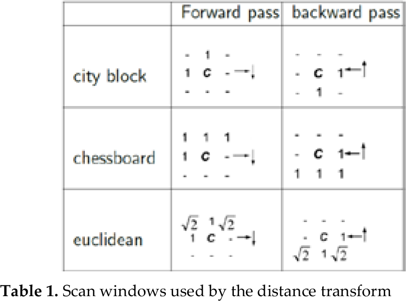
For example, let us consider a forward pass Euclidean window, w, as shown in Table 1. Let w(0,0) indicate the value of the centre cell of the Euclidean window, centred over the considered cell C = (x, y) in the map I, with a current distance value d(x, y). The new distance value for cell C is computed by the following assignment:

d (x, y) = m i n \{\begin{matrix} d (x - 1, y - 1) + w (- 1, - 1), \\ d (x, y - 1) + w (0, - 1), \\ d (x + 1, y - 1) + w (1, - 1), \\ d (x - 1, y) + w (- 1,0), \\ d (x, y) \end{matrix}

(2)

The forward pass window is moved through map I horizontally, from top left to bottom right. Then the backward pass window is moved through map I, horizontally again, but from bottom right to top left. These passes are repeated in order to propagate minimum distances on the map, until no changes are registered in matrix d(x, y). The pseudocode is shown in Algorithm 1.

Input/ – a binary map i, j – coordinates of goal Outputd a matrix with the distances until the goal Initialize d according to eq. 1 repeat for each line from the top of the map do for each cell from left to right do apply scan window 1 update d according to eq. 2 end for end for for each cell from the bottom of the map do for each line from right to left do apply scan window 2 update d according to eq. 2 end for end for until no change

Algorithm 1. Jarvis' distance transform algorithm

For an obstacle free map of X × Y cells, the complexity of Jarvis' algorithm is O(XY). The complexity of the distance transform computation can increase depending on the topology of the obstacles (which determines the required number of iterations of the repeat cycle) [16] and the execution time may vary depending on the type of scan window used.

From the distance matrix obtained by the distance transform algorithm, we can find the optimal path for a given starting point by looking at its eight neighbour cells and moving to the cell with the lowest distance value. This process is repeated until there is no neighbour cell with a lower value than the current cell, i.e., the goal cell has been reached. Since the path is found by choosing locally only between neighbour cells, the obtained path can be sub optimal, as seen in Figure 2.

Figure 2.

Sub optimal path obtained using Jarvis' approach, from s to g (top, in blue). The optimal path is shown in green.

In [16], Jarvis compares the distance transform algorithm with the A^* algorithm [17] and the Rapidly-Exploring Random Trees (RRT) approach [18] and demonstrates that the distance transform method is a good and fast algorithm. However, the paths obtained in the distance transform algorithm typically consist of a large number of small steps between neighbouring free cells, with turning angles limited to multiples of π/4.

Lee [19] describes an algorithm to generate a smoother path by grouping the small steps into a smaller number of longer and straighter segments. The path-smoothing approach starts at the first cell of the path and examines subsequent cells one at a time in order to find the farther cell that can be reached directly from the start cell in a straight movement, while remaining within free space. This cell is thus marked as a sub goal. This process is repeated until the target cell is reached. This approach can obtain smooth paths. However, it does not guarantee obtaining the optimal path. Furthermore, if we need to obtain smooth paths for every cell in the map, we need to perform this post processing for every cell as well.

3. The Exact Euclidean Distance Transform algorithm

The core of our approach, called the Exact Euclidean Distance Transform (EEDT), is that for each cell we obtain the best visible sub goal towards the goal (close to the vertices of obstacles), in order to obtain smooth paths without post-processing. We use a raster scan method, similar to the Jarvis' distance transform algorithm, due to the efficiency of such algorithms. In this way, while applying the raster scan method to update the cell's distance value d, we also keep track of the best visible sub goal p towards the goal, for each cell in the map. With the inclusion of the next-best-sub-goal matrix p, we obtain smooth paths without angle restriction. The path generated by our approach can be easily followed by an omnidirectional robot without stopping and turning at each sub-goal. For a differential robot, we need to stop and turn at each sub-goal. For a car-like robot, B-Splines can be used in order to improve the collision-free path computed by our approach.

Two cells a and b are visible to each other if the straight line segment joining the centres of these cells lies only on free cells. With this proposal, it is possible to obtain a smooth path from any point on the map to the target cell, only by following the sequence of sub-goals from any initial cell to the goal.

The operating principle of the proposed algorithm is as follows: the initial values of the matrix of transformation distance d are set in the same manner as in Jarvis' algorithm, i.e.:

d (x, y) = \{\begin{matrix} \begin{matrix} \infty, & (x, y) \neq g (x, y) \\ 0, & (x, y) = g (x, y) \end{matrix} \end{matrix}

(3)

The sub-goal matrix p is set under the following criteria:

p (x, y) = \{\begin{matrix} N U L L, & (x, y) \neq g (x, y) \\ g (x, y), & (x, y) = g (x, y) \end{matrix}

(4)

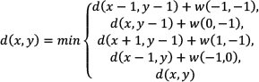
As in the Jarvis' algorithm, two raster sweeps are performed by applying a set of scan windows over the grid map. The scan windows used are shown in Figure 3. In the forward pass, scan window 1 is applied from left to right on each line, followed by the application of scan window 2 from right to left over the same line. During the backward pass, scan windows 3 and 4 are applied, line-by-line from right to left and from left to right, respectively.

Figure 3.

Windows used in our the distance transform algorithm

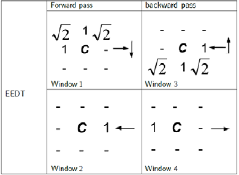
For every cell r = (x, y) marked as free in the grid map I, we analyse the v_i neighbors indicated by the scan window, verifying the visibility from r to the sub-goals assigned to each neighbour (as be discussed in Section 3.1). If from the current cell r, the sub-goal p(v_i) of the neighbouring cell is visible, the distance d_i(r) from r to the goal through the sub-goal p(v_i) is calculated, as we can see in Figure 4. If the sub-goal is not visible, then the total distance d_i(r) is calculated from r to the target passing through neighbour v_i, as shown in Figure 5 and the following expression, where w(i) is the value corresponding to neighbour i in the scan window frame w(·).

Figure 4.

Distance computation when the sub-goal of the neighbouring cell is visible.

Figure 5.

Distance computation when the sub-goal of the neighbouring cell is not visible.

d_{i} (r) = \{\begin{matrix} ||r - p (v_{i})|| + d (p (v_{i})), & p (v_{i}) i s v i s i b l e \\ w (i) + d (v_{i}), & p (v_{i}) i s n o t v i s i b l e \end{matrix}

(5)

After analysis of the neighbouring cells (determined by the scan window), if ∃d_i(r) | d_i(r) < d(r), the distance value d(r) for the current cell r is updated with the smallest of the calculated distances d_i(r) and the sub-goal p(r) is updated according to Equation 7 (p(v_i) if there is visibility and v_i if there is not visibility). In Equation 6 we show how to update d(r).

d (r) = m i n \{\begin{matrix} d (r) \\ d_{i} (r) \forall i \end{matrix}

(6)

p (r) = \{\begin{matrix} \begin{matrix} p (r), & ∄ d_{i} (r) | d_{i} (r) < d (r) \\ p (v_{i}), & \exists d_{i} (r) | d_{i} (r) < d (r) \land p (v_{i}) i s v i s i b l e \\ v_{i}, & \exists d_{i} (r) | d_{i} (r) < d (r) \land p (v_{i}) i s n o t v i s i b l e \end{matrix} \end{matrix}

(7)

The scan sequences, forward and backward, stop when there are no further changes in the matrices d and p. The pseudocode of our approach is shown in Algorithm 2.

InputI - a binary map i, j – coordinates of goal Outputd a matrix with the distances up to the goal p a matrix with the next subgoal Initialize d according to eq. 3 and p according to eq. 4 repeat for each line from the top of the map do for each cell from left to right do apply scan window 1 update d and p according to eq. 6 and 7 end for for each cell from right to left do apply scan window 2 update d and p according to eq. 6 and 7 end for end for for each line from the bottom of the map do for each cell from right to left do apply scan window 3 update d and p according to eq. 6 and 7 end for for each cell from left to right do apply scan window 4 update d and p according to eq. 6 and 7 end for end for until no change

Algorithm 2. Exact Euclidean Distance Transform algorithm

3.1 Visibility test

In order to assign a valid (visible) sub goal, we proceed in two steps. First, we chose the two neighbours closer to the line of vision we want to verify. If the same sub goal is assigned to the two neighbours, then both neighbours can “see” the sub goal and the line of vision between the actual cell r = (x, y) and the sub goal is collision-free (Figure 6). Indeed, p(v_a) = p(v_b) = p(v_i) and this sub goal can be assigned to the actual cell. On the other hand, when the sub goals of the two neighbours are different (p(v_a) ≠ p(v_i) V p(v_b) ≠ p(v_i)), then it is necessary to verify the whole line of vision (Figure 7). The straight line is calculated by means of Bresenham's line algorithm [20]. The pseudocode for assigning a valid sub goal is shown in Algorithm 3.

Figure 6.

The same sub goal is assigned to the two neighbours

Figure 7.

The sub goals of the two neighbours are different

Inputp(v_i) - the target point Outputtrue - If visibility exists false - If not visibility exists Identify the v_a and v_b nearest neighbors to the straight line to the goal if p(v_a) = p(v_b) = p(v_i) then the cell pointed by the neighbour is visible else check vision line using the Bresenham's algorithm end if

Algorithm 3. Visibility test

In our approach, we build two matrices: the first one contains the Euclidean distance from each cell to the target (value d) and the second one contains, for each cell, the best visible sub goal (next cell p) towards the target. The shortest path can be computed by selecting any starting point (x, y) on the map and then tracing to the next point p(x, y). The first step in the optimal plan to the goal can be determined by Equations 6 and 7, which yields a new state p‘(x, y) and d’(r). From p‘(x, y) and d’(r), Equations 6 and 7 can be applied once again to determine the next optimal action. The cost at d‘(r) and the sub goal at p’(x, y) represents both the optimal cost-to-go if (x, y) is the initial condition and also the optimal cost-to-go when continuing on the optimal path from (x, y).

For an obstacle free environment of X × Y cells, the complexity of our algorithm is, at worst (when all lines of vision must be verified), O(X²Y). Like for Jarvis' distance transform, the complexity of the distance transform computation can increase depending on the topology of the obstacles (which determines the required number of iterations of the repeat cycle).

4. Numerical results

We compared our EEDT algorithm with other distance transform algorithms proposed by Jarvis using different windows: City block, Chessboard and Euclidean. Moreover, we implemented the path smoothing method proposed in [18] for each one of Jarvis' algorithms. Also, we solve the path-planning problem with a visibility graph approach. Since the visibility graph works only on roadmaps, the graph is built using the detected corners in the grid map. To carry out our experiments, the system was tested in different scenarios, with different goal points, in order to analyse how the approach copes in different environments. We checked the execution speed, the accuracy of the resulting distance and the number of sub goals from a starting point up to the goal. The different environments used in our experiment are shown in Figure 8.

Figure 8.

Maps used for the test.

4.1 Obtained paths

Figure 9 shows the comparative results of the obtained paths by applying the distance transformation algorithms. Figures 9(a), 9(b) and 9(c) show the paths obtained when using Jarvis' algorithm with the scan windows City block, Chessboard and Euclidean respectively and in which we see that for the generated paths, the angle of displacement is limited to multiples of π/4.

Figure 9.

Paths obtained for the “autolab” map (405 × 345 pixels).

Figures 9(d), 9(e) and 9(f) show the results obtained by applying the path-smoothing algorithm proposed by Lee [18], in which the angle displacement is not limited to multiples of π/4. However, there is no guarantee that the generated path will be optimal. Finally, our approach produces smooth paths, whose total length is close to optimal and is similar to the shortest-paths obtained with the visibility graph approach (Figure 9(h)), without the need of any post-processing. In Figure 9(g) we can see the paths generated by our approach.

Observing Figure 9(g), we can see that the generated trajectories using our algorithm always select sub-goals near to the obstacles vertices. In addition, at every step of the way we know the position of the next sub-goal visible from the current position.

These results clearly show that our approach, by keeping track of the visible sub-goals with matrix p, is very efficient in constructing trajectories towards the goal and includes detailed information of the Euclidean distance toward the target.

In concrete terms, our algorithm constructs a visibility map of the environment, as shown in Figure 10, where each sub-region has a visible goal for all points within that region. In Figure 10, an arrow indicates the best local sub-goal visible for each region.

Figure 10.

Best local sub-goal for some maps. For each region (colour) the arrows point to the next sub-goal.

4.2 Distances evaluation

In order to compare the distances obtained by our algorithm against the various distance transform approaches, we compute the relative error between them. We used an obstacle-free environment where the wave front is generated from a single point in the centre of the map and we compute the root mean squared error (RMSE). Moreover, we test the accuracy in the environments shown in Figure 8, with the wave front generated from different points and we compute the RMSE and the worst error mean.

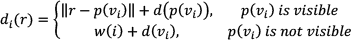
For an obstacle-free environment, the worst results are obtained by Jarvis' approach, however Jarvis' approach with post-processing give errors equal to zero, as in our approach (refer to the Appendix A). The result of a perfect distance transform should be circular. Figure 11 demonstrates that our approach and Jarvis' approach (with path smoothing) generate circular waves in obstacle-free environments, in which the grey scale of each cell is proportional to the distance to the target.

Figure 11.

Resulting images for an obstacle-free map (1000 × 1000 pixels). The grey scale of each cell represents the distance to the target.

However, in maps with obstacles (Figure 12 and 13) the only algorithm that generates smooth rounded wave fronts is our approach, whereas Jarvis' approach obtained results without rounded borders. On the other hand, Jarvis' approach with path-smoothing post-processing obtains a wave front with rounded borders, but with some errors in the computed distance, as can see by the broken profile of the wave front (Figure 12(d), 12(e), 12(f), as well as Figure 13(d), 13(e) and 13(f)).

Figure 12.

Resulting images for “autolab” map (405 × 345 pixels). The grey scale of each cell represents the distance to the target.

Figure 13.

Resulting images for “cave” map (400 × 400) pixels. The grey scale of each cell represents the distance to the target.

These results are given in Appendixes B and C, which present the relative errors of Jarvis' method compared to our algorithm. These errors are all positive, since our algorithm computes the shortest distances to the goal. The worst results are obtained by Jarvis' approach, which can be improved by post-processing (in some cases the errors are close to zero). However, applying the smoothing algorithm on the results of the algorithm proposed by Jarvis considerably increases the computation time compared to our approach, as we can see in Appendix D.

The resulting images for some maps are shown in Figures 12 and 13 and we can appreciate the different profiles between the wave fronts generated by our algorithm and the other algorithms.

4.3 Execution times

In order to determine the execution speeds, all algorithms were tested on the maps shown in Figure 8, with the wave fronts generated from different starting points. For each tested point, the execution times were averaged over 31 iterations. The average times required by our approach are slightly more important than those required for Jarvis' approach without post processing. However, in order to obtain comparable wave fronts, it is necessary to apply, to the Jarvis' algorithm results, the path-smoothing algorithm proposed by Lee. Thereby, it increases the execution time compared to our proposal (Appendix D).

5. Conclusions

This paper presents a new raster scan method for computing the Euclidean distance transform, in order to obtain a universal path planner for mobile robots, which solves the needs to obtain accurate distances toward goals and to generate smooth trajectories for some exploration algorithms. Besides obtaining the distance to the goal for every cell in the map, we obtain the next visible sub goal and consequently we can generate a good short and smooth path without post processing, similar to the one obtained using the visibility graph approach. From the numerical comparison of the obtained paths (for various distance transform algorithms), we demonstrate that our approach has great efficiency in computing a sequence of sub-goals from any starting point up to the goal. Also, the proposed approach has no restriction on the angle turn, as in Jarvis' algorithms. Finally, our approach does not need a bulky overhead computation to keep track of the best visible sub-goals: the visibility from the neighbour cells is exploited in order to add efficiency to our algorithm.

Footnotes

6. Appendixes

References

Yamauchi

(1997). A frontier-based approach for autonomous exploration. CIRA '97: Proceedings of the 1997 IEEE International Symposium on Computational Intelligence in Robotics and Automation, page 146, Washington, DC, USA.

Elizondo-Leal

J C

Ramírez-Torres

and Pulido

G Toscano

(2008). Multi-robot exploration and mapping using self biddings and stop signals. MICAI, Lecture Notes in Computer Science Springer, 5317: 615–625.

Burgard

Moors

Stachniss

and Schneider

(2005). Coordinated multi-robot exploration. IEEE Transactions on Robotics and Automation, 21: 376–386.

Lozano-Perez

and Wesley

(1979). An Algorithm for Planning Collision-free Paths among Polyhedral Obstacles. Communication of the ACM, 22: 560–570.

Xiao

Michalewicz

Zhang

and Trojanowski

(1997). Adaptive evolutionary planner/navigator for mobile robots. IEEE Transactions on Evolutionary Computation, 1: 18–28

Bylander

(1994). The computational complexity of propositional STRIPS planning. Artificial Intelligence, 69 (1-2): 165–204.

Masehian

and Sedighizadeh

(2007). Classic and heuristic approaches in robot motion planning-a chronological review. World Academy of Science, Engineering and Technology, 23: 101–106

Meyer

J A

and Filliat

(2003). Map-based navigation in mobile robots. ii. a review of map-learning and path-planning strategies. Cognitive Systems Research, 4 (4): 283–317.

Schoppers

(1987). Universal plans for reactive robots in unpredictable environments. IJCAI: 1039–1046.

10.

Latombe

J C

(1991). Robot Motion Planning. Kluver Academic Publishers, Boston, MA.

11.

Elizondo-Leal

J C

and Ramírez-Torres

(2010). An Exact Euclidean Distance Transform for Universal Path Planning. Cerma, 2010 IEEE Electronics, Robotics and Automotive Mechanics Conference: 62–67

12.

Khatib

(1986). Real-time obstacle avoidance for manipulators and mobile robots. The International Journal of Robotics Research, 5 (1): 90–99.

13.

Barraquand

Langlois

and Latombe

(1992). Numerical potential field techniques for robot path planning. IEEE Transactions on Systems, Man and Cybernetics, 22 (2): 224–241.

14.

Jarvis

R A

(1985). collision-free trajectory planning using distance transform. Proc. National Conference and Exhibition on Robotics, Melbourne, 20-24th Aug. 1984, also in Mechanical Engineering Transactions, Journal of the Institution of Engineers, ME 10 (3): 187–191.

15.

Rosenfeld

and Pfaltz

(1966). Sequential operations in digital picture processing. Journal of the ACM, 13 (4): 471–494.

16.

Jarvis

(2006). Robot path planning: complexity, flexibility and application scope. PCAR '06: Proceedings of the 2006 international symposium on Practical cognitive agents and robots: 3–14.

17.

Lozano-Pérez

and Wesley

M A

(1979). An algorithm for planning collision-free paths among polyhedral obstacles. Commun. ACM, 22: 560–570.

18.

Lavalle

S M

(1998). Rapidly-exploring random trees: A new tool for path planning. Technical report.

19.

Lee

(1996). The map-building and exploration strategies of a simple sonar-equipped mobile robot. Cambridge University Press, New York, NY, USA.

20.

Bresemham

(1987). Ambiguities in incremental line rastering. IEEE Comput. Graph. Appl., 7: 31–43.