Visual Servoing Tracking Control of a Ball and Plate System: Design,Implementation and Experimental Validation

Abstract

This paper presents the design, implementation and validation of real-time visual servoing tracking control for a ball and plate system. The position of the ball is measured with a machine vision system. The image processing algorithms of the machine vision system are pipelined and implemented on a field programmable gate array (FPGA) device to meet real-time constraints. A detailed dynamic model of the system is derived for the simulation study. By neglecting the high-order coupling terms, the ball and plate system model is simplified into two decoupled ball and beam systems, and an approximate input-output feedback linearization approach is then used to design the controller for trajectory tracking. The designed control law is implemented on a digital signal processor (DSP). The validity of the performance of the developed control system is investigated through simulation and experimental studies. Experimental results show that the designed system functions well with reasonable agreement with simulations.

1. Introduction

A ball and plate system is a common experimental setup in control laboratories. It consists of a horizontal plate, which is tilted along each of two horizontal axes such that a ball can be controlled to roll to any position on the plate. It serves to visually demonstrate and reinforce the underlying principles of nonlinear dynamics and control theory. Moreover, because of its inherent nonlinearity, instability, and underactuation, this system is widely used as a test bed for verifying the performance and effectiveness of new control algorithms or technology. Several aspects of mechatronic design, implementation, and control of a ball and plate system have been investigated in the literature [1-10]. In existing studies, the control design has usually been based on the simplified model of the ball and plate system, and derivation of a detailed dynamic model has received far less attention. Based on the model linearized with respect to the equilibrium, [1] designed a PID controller and lead controller to stabilize the system. In [3, 7], a nonlinear simplified model was given, and a sliding mode control was used to achieve trajectory tracking. Based on a linear simplified model, [10] designed a PID controller and state observer feedback controller to achieved set-point regulation and trajectory tracking.

For a ball and plate system, sensors for sensing the position of the ball can be divided into two main types: the touch screen [1, 10] and the overhead camera [2-6, 8, 9]. Both these sensing devices suffer from certain shortcomings. The ball can easily lose contact with the touch screen plate during the motion, and this causes discontinuity in the position measurement. Since the sampling rate of a common camera (30 Hz) is limited, use of a common camera for sensing the position of the ball imposes real-time constraints on the system. Visual servoing [11] is a control framework that incorporates visual information in feedback control loops. Real-time image data acquisition and processing is a critical issue in visual servoing applications. A high frame rate and low processing latency are essential since the visual servoing system must make quick decisions based on the information extracted from a scene. Real-time image processing requires a high pixel processing rate, massive and parallel computation, and efficient hardware utilization. General-purpose processors cannot always provide enough computational power to fulfil real-time requirements due to their sequential nature. Due to their inherent architectural parallelism and configurable flexibility, field programmable gate arrays (FPGAs) have become increasingly popular implementation platforms for real-time image processing. In [12], an FPGA/DSP (digital signal processor) architecture was proposed for real-time image processing. This architecture was designed to deal with parallel/pipelined procedures to handle multiple input images. A flexible FPGA-based systolic architecture for real-time window-based image processing was proposed in [13]. Its computational core was based on a configurable two-dimensional systolic array of processing elements. In [14, 15], FPGAs with a pipelined architecture were used to implement optical flow estimation from image sequences in real time.

The idea behind feedback linearization [16-18] is to find a diffeomorphism and a state feedback control law that transform the nonlinear system into a linear time-invariant system. The design is then carried out on the linear system using linear control design techniques. Both full-state feedback linearization and partial-state feedback linearization can be considered. In full-state feedback linearization, also called input-state feedback linearization, the state equations are fully linearized. In partial-state feedback linearization, also called input-output feedback linearization, the input-output map of the system is linearized, while the map from the input to the state can be only partially linearized. However, the applicability of feedback linearization is limited to special classes of nonlinear systems satisfying the constraints of controllability, involutivity, and the existence of a relative degree or minimum phase property. One approach to relaxing one or more of these applicability constraints is to use the techniques of approximate feedback linearization. Approximate feedback linearization was first proposed in [19], where necessary and sufficient conditions for approximate full-state feedback linearization of nonlinear systems are given. This method is intended to find a nonlinear coordinate change and state feedback such that a linear approximation is obtained for an equilibrium point accurate to second or higher order. In [20], it was shown that one can approximately input-output linearize a nonlinear system by neglecting the nonlinearities responsible for the failure of the involutivity conditions. An approximate tracking controller was then designed for a ball and beam system.

This paper presents the design, implementation, and validation of tracking control of a ball and plate system using visual feedback. The position of the ball is measured with a machine vision system that uses an image sensor with a frame rate of 150 frames per second to guarantee a certain level of real-time performance. The pipelined image processing of the machine vision system is implemented on an FPGA device to meet real-time constraints. The detailed dynamic model of the ball and plate system is derived. This detailed dynamic model is adopted to build a reliable and accurate simulation model for the purpose of validating the closed-loop performance of the control system, once a controller design is available. For control design purposes, the detailed dynamic model is far too complex. By neglecting the high-order coupling terms, the ball and plate system is simplified into two decoupled ball and beam systems, and an approximate input-output feedback linearization approach [20] is then used to design a controller for trajectory tracking. A DSP is used for the implementation of the control algorithm and complex arithmetic operations. The effectiveness of the controller and machine vision system is validated through simulation and experimental results. Some studies [8, 9] have reported the control of a vision-based ball and plate system via an FPGA implementation. The processing frame rate of the machine vision system developed in this paper (150 frames/sec) is much higher than that of [8] and [9] (16 frames/sec). Unlike the present work, the experimental results given in [8] and [9] are the results of set-point regulation, which is less challenging.

The rest of this paper is organized as follows. In Section 2, a brief description of the experimental setup is given. Section 3 describes the relationship between the world coordinates and the image coordinates. The image processing algorithms for determining the position of the ball from the image data are introduced, and the implementation and architecture of the image processing algorithms on an FPGA device are presented. In Section 4, the dynamic model of a ball and plate system is derived. In Section 5, a review of approximate input-output feedback linearization is presented. Based on approximate input-output feedback linearization, the design of a controller for trajectory tracking is given. In Section 6, the simulation and experimental results are given. Finally, Section 7 contains some concluding remarks.

2. Experimental Apparatus

The experimental setup of a ball and plate system is shown in Figure 1, and the schematic overview of the experimental setup is shown in Figure 2. The system consists of two dc motors with gear heads. Each motor shaft is fixed to an L-shaped linkage that is attached to the plate with a universal joint. This L-shaped linkage consists of two linkages connected with a bearing joint. The plate is pivoted at its centre with a universal joint. When the L-shaped linkage is driven by the motor to move up and down, the plate inclines and changes its rotational angles; thus the ball can roll on the plate. This actuation mechanism is similar to the one designed and implemented in [1]. An optical encoder with a resolution of 1250 pulses/rev is attached to each motor shaft to measure the angular position of the motor. The position of the ball is measured with an overhead machine vision system, which consists of a CMOS camera sensor, static random access memory (SRAM), and an FPGA board. The camera is a Micron CMOS image sensor, MT9M011, which can capture 352×288 pixels quantized to 1024 RGB-colour-levels at 160 frames per second. In this study, the image sensor is set to operate in the grey-level mode at 150 frames per second. The SRAM (13M bits) acts as a frame buffer, which is used for storing an image during camera calibration. An FPGA board is used to implement the image processing algorithms written in very-high-speed integrated circuit hardware description language (VHDL). The FPGA board is an Altera Cyclone EP1C12Q240C8 FPGA. The controller is implemented on a DSP board, which is the Texas Instruments TMS320F240 digital signal processor (150-MHz/32-bit) equipped with two 12-bit D/A converters and two quadrature encoder pulse (QEP) units. The QEP unit provides the angular position and rotational direction of the motor from the quadrature encoder signals. The velocity of the ball and the angular velocity of the motors are estimated from the displacement travelled per unit time, and then the estimated velocities are passed through digital low-pass filters to attenuate the high-frequency noise. Voltage signals are generated according to the designed control law and supplied to the power amplifiers that drive the dc motors. The power amplifiers are operational amplifiers that can operate at up to ±20 V and 2.75 A.

Figure 1.

Experimental setup of the ball and plate system.

Figure 2.

Schematic diagram of the experimental setup.

3. Visual Measurement and Image Processing Algorithm

A machine vision system is used to determine the displacement of the ball on the plate. A black ball and white plate are used to simplify visual sensing and to increase the accuracy of visual measurements. Determination of the position of the ball is based on the perspective pinhole camera model [21-22], which is given by

$\lambda p=K_I [R_E | t] P_O,$

(1)

where p = [x_im, y_im, 1]^T represents the two-dimensional homogeneous coordinates of the image point in the image coordinate system; P_O = [X, Y, Z, 1]^T represents the three-dimensional homogeneous coordinates of the object point in the world coordinate system, and λ is a scalar factor. The 3×3 matrix R_E and three-dimensional vector t are extrinsic camera parameters that describe the rotation and translation between the world frame and the camera frame, respectively. K_I is the intrinsic camera parameter matrix given by

$K_I=\left[\begin{array}{ccc}{f}_{sx}& f_{s\theta }& o_x\\ 0& f_{sy}& o_y\\ 0& 0& 1\end{array}\right].$

(2)

Here, (o_x, o_y) is the principal point on the image coordinate system in pixels; f_sx is the size of the unit length in horizontal pixels; f_sy is the size of the unit length in vertical pixels, and f_sθ is the skew of the pixels. The world frame oXYZ is chosen with the Z-axis pointing vertically upwards and the origin o located at the centre of the plate. The camera is mounted right above the plate with its optical axis passing through the origin of the world frame. The camera frame is denoted by o_cx_cmv_cmz_cm. Th x_cm-axis of the camera frame is chosen to be parallel and aligned to the X-axis of the world frame. Thus, the ycm-axis points vertically downwards. The extrinsic camera parameters are then given by:

$[R_E|t]=\left[\begin{array}{cccc}1& 0& 0& 0\\ 0& -1& 0& 0\\ 0& 0& -1& d_c\end{array}\right],$

(3)

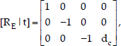
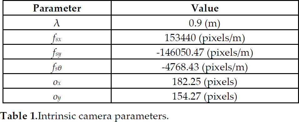
where d_c = 0.91 (m) is the distance from the origin of the world frame to the origin of the camera frame. The intrinsic camera parameters are obtained using the camera calibration procedure proposed in [21]. In this study, the parameter λ = d_c – R is obtained, where R is the radius of the ball. The intrinsic camera parameters are given in Table 1.

Table 1.

Intrinsic camera parameters

Parameter	Value
λ	0.9 (m)
fsx	153440 (pixels/m)
fsy	−146050.47 (pixels/m)
fsθ	−4768.43 (pixels/m)
ox	182.25 (pixels)
oy	154.27 (pixels)

To determine the position of the ball on the image plane, the captured images are processed using a series of image processing algorithms. A sample of a raw image captured by the camera is shown in Figure 3.

Figure 3.

Image captured by the camera.

The image processing algorithm steps [23] are described below:

Step 1. Background subtraction

Background subtraction is an approach to differentiate foreground objects from their background. This step is used here to remove brightness fluctuations due to uneven background illumination. Background subtraction was applied to the image in Figure 3 and the resulting image is shown in Figure 4.

Figure 4.

Background subtraction applied to the image in Fig. 3.

Step 2. Thresholding

Thresholding is a simple and efficient method applied to grey-level intensity images to differentiate between the object and the background. Moreover, thresholding converts a grey-scale image into a bi-level image which contains all of the essential information concerning the shape, position and number of objects. This process is described as follows:

$f(x_{im},y_{im})=\{\begin{array}{c}\begin{array}{cc}255& \text{if }f(x_{im},y_{im})\ge T_{th}\end{array}\\ \begin{array}{cc}0 & if f(x_{im},y_{im})<T_{th}\end{array}\end{array},$

(4)

where f(x_im,y_im) is the grey-scale level of the pixel at point (x_im,y_im) in the image coordinate system, and T_th is the threshold value. Applying thresholding with a threshold value of 100 to the image in Figure 4 produces the image in Figure 5. The threshold value is determined experimentally to obtain the best system performance.

Figure 5.

Thresholding applied to the image in Fig. 4.

Step 3. Median filter

As seen in Figure 5, there is noise in the image. Further filtering processing is needed to remove noise. Noise removal is performed by a median filter, which requires the use of a 3×3window to slide along the image, and the median intensity value of the pixels within the window becomes the output intensity of the centre pixel. Applying the median filtering process to the image in Figure 5 produces the image in Figure 6.

Figure 6.

Median filtering process applied to the image in Fig. 5.

Step 4. Centroid determination

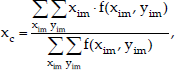
As shown in Figure 6, the white pixels correspond to the ball, while the plate is shown by the black pixels. Since the ball is symmetrical, the centroid of the image of the ball is taken as its location on the plate. The centroid (x_c, y_c) is given by

$x_c=\frac{{\displaystyle \sum _{x_{im}}{\displaystyle \sum _{y_{im}}{x}_{im}\cdot f(x_{im}, y_{im})}}}{{\displaystyle \sum _{x_{im}}{\displaystyle \sum _{y_{im}}f(x_{im}, y_{im})}}},$

(5)

$y_c=\frac{{\displaystyle \sum _{x_{im}}{\displaystyle \sum _{y_{im}}{y}_{im}\cdot f(x_{im}, y_{im})}}}{{\displaystyle \sum _{x_{im}}{\displaystyle \sum _{y_{im}}f(x_{im}, y_{im})}}}.$

(6)

In order to process the image data in real time, the image processing algorithms are implemented on an FPGA using VHDL. The FPGA technology is chosen because it is able to provide massive amounts of reprogrammable hardware acceleration and parallel/pipelined processing ability. In this study, the image processing is divided into the modules as shown in Figure 7.

Figure 7.

FPGA architecture pipelined.

The functions of the modules are:

• M₁: The Inter-Integrated Circuit(I²C) serial interface is used to configure the frame rate, gain control, exposure time, and integration time of the camera.

• M₂: The frame grabber module acquires the pixels at a rate of 25 Mbytes/sec from the camera. The image data can be directly passed to the next module or stored in external SRAM for camera calibration.

• M₃: This module is designed to realize background subtraction. The grey-scale level of the background image pixel is subtracted from the incoming pixel.

• M₄: This module applies thresholding to the output image of the background subtraction stage. Since after background subtraction the ball has higher intensity than the plate in the image, the thresholding method is used to differentiate the ball from the background.

• M₅: Median filtering is performed on the output image of the thresholding stage to reduce noise.

• M₆: The centroid of the ball (Equations (5) and (6)) is calculated in this stage.

There is no iterative process in this design. Thus, this processing can be fully pipelined in hardware implementation to improve efficiency and provide a high data throughput rate. The design is implemented on Altera Cyclone EP1C12Q240C8 FPGA. The FPGA configuration data is stored in an electrically-erasable programmable read-only memory (EEPROM) and can be re-programmed by the host computer. A programmable clock generator is used to generate three global clocks for system clocks and the pixel clock. The I²C serial interface is set to operate at 62.5 kHz; the operation frequency for carrying out image processing is 100 MHz, and the pixel clock is also 100 MHz. In order for the DSP board to communicate with the FPGA, a 16-bit bus connected to the DSP board data bus is used for data exchange. The read/write commands are specified with different addresses. The proposed design can process 150 grey-level images per second with a resolution of 352 × 288 pixels.

4. System Modelling

In this section, we derive the mathematical model of the ball and plate system by using the Euler-Lagrange method [24]. Figure 8 illustrates the basic features of the system. Assuming that the ball rolls on the plate without slipping, the ball is always in contact with the plate; there is no rotational motion of the ball with respect to its vertical axis, and all friction forces and torques are neglected. There are two coordinate frames used, as shown in Figure 8.

Figure 8.

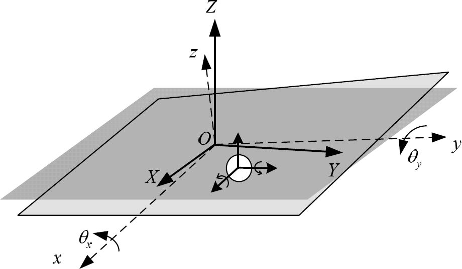
Coordinate frames for the ball and plate system.

The space-fixed coordinate system (world frame) oXYZ has the Z-axis pointing vertically upwards and the origin located at the centre of the plate. Unit vectors along the oXYZ-coordinate system are denoted by Î, Ĵ, and K̂. The coordinate system fixed on the plate with the z-axis perpendicular to the plate and the origin located at the centre of the plate is denoted by oxyz. Unit vectors along the oxyz-coordinate system are denoted by î, ĵ, and K̂. The oxyz-coordinate system is, with respect to the oXYZ-coordinate system, rotated about the x-axis by an angle θ_x followed by a rotation about the y-axis by an angle θ_y. The Euler-Lagrangian equation is

$\frac{d}{dt}\left[\frac{\partial L}{\partial \stackrel{.}{q}}\right]-\frac{\partial L}{\partial q}=Q\text{,}$

(7)

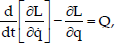
where L is the Lagrangian function, and Q and q are the generalized forces and generalized coordinates, respectively. The Lagrangian function L is defined as

$L=T-V\text{,}$

(8)

where T is the kinetic energy, and V is the potential energy. For this system, q is selected as

$q=\left[\begin{array}{c}x\\ y\\ {\theta }_x\\ {\theta }_y\end{array}\right],$

(9)

Q is given by

$Q=\left[\begin{array}{c}0\\ 0\\ {\tau }_x\\ {\tau }_y\end{array}\right],$

(10)

where τ_x and τ_y are the torques exerted on the plate in the x-axis and y-axis, respectively.

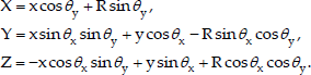
If the inclination of the plate changes, the ball moves on the plate. The position of the ball relative to the plate-fixed coordinate can be mapped into the space-fixed coordinate. The transformation between these coordinates is written as follows:

$\left[\begin{array}{l}x\\ y\\ z\end{array}\right]={\hspace{0.17em}}^{P}R{}_F\left[\begin{array}{l}X\\ Y\\ Z\end{array}\right],$

(11)

where ^PR_F is the rotation matrix and

${\hspace{0.17em}}^{P}R{}_F=\left[\begin{array}{ccc}\cos {\theta }_y& \sin {\theta }_x\sin {\theta }_y& -\cos {\theta }_x\sin {\theta }_y\\ 0& \cos {\theta }_x& \sin {\theta }_x\\ \sin {\theta }_y& -\sin {\theta }_x\cos {\theta }_y& \cos {\theta }_x\cos {\theta }_y\end{array}\right].$

(12)

The position vector of the ball in the oxyz -coordinate system is given by

$\widehat{r}=x\widehat{i}+y\widehat{j}+R\widehat{k},$

(13)

where R is the radius of the ball. From (11), we have

$\begin{array}{l}X=x\cos {\theta }_y+R\sin {\theta }_y,\\ Y=x\sin {\theta }_x\sin {\theta }_y+y\cos {\theta }_x-R\sin {\theta }_x\cos {\theta }_y,\\ Z=-x\cos {\theta }_x\sin {\theta }_y+y\sin {\theta }_x+R\cos {\theta }_x\cos {\theta }_y.\end{array}$

(14)

By taking derivative of (14) with respect to time, the velocity vector of ball in the oXYZ -coordinate system is then given by

$\widehat{v}=\stackrel{.}{X}\widehat{I}+\stackrel{.}{Y}\widehat{J}+\stackrel{.}{Z}\widehat{K},$

(15)

where

$\stackrel{.}{X}=\stackrel{.}{x}\cos {\theta }_y-x{\stackrel{.}{\theta }}_y\sin {\theta }_y+R{\stackrel{.}{\theta }}_y\cos {\theta }_y\text{,}$

(16)

$\begin{array}{l}\stackrel{.}{Y}=\stackrel{.}{x}\sin {\theta }_x\sin {\theta }_y+\stackrel{.}{y}\cos {\theta }_x-y{\stackrel{.}{\theta }}_x\sin {\theta }_x\\ +x({\stackrel{.}{\theta }}_x\cos {\theta }_x\sin {\theta }_y+{\stackrel{.}{\theta }}_y\sin {\theta }_x\cos {\theta }_y) \\ -R({\stackrel{.}{\theta }}_x\cos {\theta }_x\cos {\theta }_y-{\stackrel{.}{\theta }}_y\sin {\theta }_x\sin {\theta }_y)\text{,}\end{array}$

(17)

$\begin{array}{l}\stackrel{.}{Z}=-\stackrel{.}{x}\cos {\theta }_x\sin {\theta }_y+\stackrel{.}{y}\sin {\theta }_x+y{\stackrel{.}{\theta }}_x\cos {\theta }_x\\ -x(-{\stackrel{.}{\theta }}_x\sin {\theta }_x\sin {\theta }_y+{\stackrel{.}{\theta }}_y\cos {\theta }_x\cos {\theta }_y) \\ +R(-{\stackrel{.}{\theta }}_x\sin {\theta }_x\cos {\theta }_y-{\stackrel{.}{\theta }}_y\cos {\theta }_x\sin {\theta }_y).\end{array}$

(18)

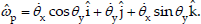
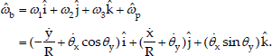
The angular velocity vector of the plate due to rotation is denoted by

${\widehat{\omega }}_p={\omega }_{px}\widehat{i}+{\omega }_{py}\widehat{j}+{\omega }_{pz}\widehat{k}.$

(19)

The relation between the rotation matrix and angular velocity [24] is given as

${\hspace{0.17em}}^{P}R{}_F{({\hspace{0.17em}}^P\stackrel{.}{R}{}_F)}^{\mathrm{T}}=\left[\begin{array}{ccc}0& -{\omega }_{pz}& {\omega }_{py}\\ {\omega }_{pz}& 0& -{\omega }_{px}\\ -{\omega }_{py}& {\omega }_{px}& 0\end{array}\right].$

(20)

From (20) and (12), it is given that

${\widehat{\omega }}_p={\stackrel{.}{\theta }}_x\cos {\theta }_y\widehat{i}+{\stackrel{.}{\theta }}_y\widehat{j}+{\stackrel{.}{\theta }}_x\sin {\theta }_y\widehat{k}.$

(21)

Let ω₁^î+ω₁^ĵ +ω₁^K̂ denote the angular velocity vector of the ball with respect to the oxyz-coordinate system. Under the assumption of rolling without slipping and twisting we have the following conditions:

$\begin{array}{l}{\omega }_1=-\frac{\stackrel{.}{y}}{R},\\ {\omega }_2= \frac{\stackrel{.}{x}}{R},\\ {\omega }_3= 0.\end{array}$

(22)

Let ${\widehat{\omega }}_b$ be the angular velocity vector of the ball relative to the oXYZ-coordinate system. Since both the plate and ball are rotating, ${\widehat{\omega }}_b$ is the sum of the angular velocity of the ball relative to the plate and the angular velocity of the plate. Thus, from (21) and (22), ${\widehat{\omega }}_b$ is given by

$\begin{array}{l}{\widehat{\omega }}_b={\omega }_1\widehat{i}+{\omega }_2\widehat{j}+{\omega }_3\widehat{k}+{\widehat{\omega }}_p\hfill \\ =(-\frac{\stackrel{.}{y}}{R}+{\stackrel{.}{\theta }}_x\cos {\theta }_y) \widehat{i}+(\frac{\stackrel{.}{x}}{R}+{\stackrel{.}{\theta }}_y)\widehat{j}+({\stackrel{.}{\theta }}_x\sin {\theta }_y) \widehat{k}.\hfill \end{array}$

(23)

The kinetic energy of the ball is given by

$\begin{array}{l}{T}_{ball}=\frac{1}{2}m\widehat{v}\cdot \widehat{v}+\frac{1}{2}{J}_b{\widehat{\omega }}_b\cdot {\widehat{\omega }}_b\hfill \\ =\frac{1}{2}m({\stackrel{.}{X}}^2+{\stackrel{.}{Y}}^2+{\stackrel{.}{Z}}^2)\hfill \\ +\frac{1}{2}{J}_b[{(-\frac{\stackrel{.}{y}}{R}+{\stackrel{.}{\theta }}_x\cos {\theta }_y)}^2\hfill \\ +{(\frac{\stackrel{.}{x}}{R}+{\stackrel{.}{\theta }}_y)}^2+{({\stackrel{.}{\theta }}_x\sin {\theta }_y)}^2],\hfill \end{array}$

(24)

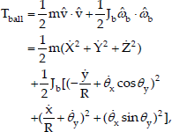
where m and J_b are the mass and moment of inertia of the ball, respectively. Let the inertia matrix of the plate be

${\mathrm{J}}_{\mathrm{p}}=\left[\begin{array}{ccc}{\mathrm{J}}_{\text{px}}& 0& 0\\ 0& {\mathrm{J}}_{\text{py}}& 0\\ 0& 0& {\mathrm{J}}_{\text{pz}}\end{array}\right],$

where J_px, J_py, and J_pz are the moment of inertia about the x, y, and z-axes, respectively. The kinetic energy of the plate is then given by

$\begin{array}{l}{T}_{plate}=\frac{1}{2}[{\omega }_{px} {\omega }_{py} {\omega }_{pz}] J_p\left[\begin{array}{c}{\omega }_{px}\hfill \\ {\omega }_{py}\hfill \\ {\omega }_{pz}\hfill \end{array}\right]\hfill \\ =\frac{1}{2}[J_{px}{({\stackrel{.}{\theta }}_x\cos {\theta }_y)}^2+J_{py}{({\stackrel{.}{\theta }}_y)}^2+J_{pz}{({\stackrel{.}{\theta }}_x\sin {\theta }_y)}^2].\hfill \end{array}$

(25)

Then, the total kinetic energy of the system is

$T=T_{ball}+T_{plate}.$

(26)

From (14), the potential energy of system is given by

$\begin{array}{l}V=mgZ\hfill \\ =mg[-x\cos {\theta }_x\sin {\theta }_y+y\sin {\theta }_x\hfill \\ +R\cos {\theta }_x\cos {\theta }_y],\hfill \end{array}$

(27)

where g is the gravitational acceleration. By using (8), (26) and (27), the Lagrangian function is given by

$\begin{array}{l}L=\left(\frac{m{R}^2+J_b}{2R^2}\right){\stackrel{.}{x}}^2+\left(\frac{m{R}^2+J_b}{2R^2}\right){\stackrel{.}{y}}^2\\ +\frac{1}{2}\left(J_b+J_{py}+m{R}^2+m{x}^2\right){\stackrel{.}{\theta }}_y{}^2-m\stackrel{.}{x}y{\stackrel{.}{\theta }}_x\sin {\theta }_y\\ +\frac{1}{4}(2J_b+2J_{px}{\cos }^2{\theta }_y+2J_{pz}{\sin }^2{\theta }_y+m{R}^2+m{x}^2\\ + 2m{y}^2+(m{R}^2-m{x}^2)\cos 2{\theta }_y-2mRx\sin 2{\theta }_y){\stackrel{.}{\theta }}_x{}^2\\ +\left(\frac{mRx\sin {\theta }_y-(J_b+m{R}^2)\cos {\theta }_y}{R}\right){\stackrel{.}{\theta }}_x\stackrel{.}{y}\\ -my\left(x\cos {\theta }_y+R\sin {\theta }_y\right){\stackrel{.}{\theta }}_x{\stackrel{.}{\theta }}_y+\left(\frac{J_b+m{R}^2}{R}\right){\stackrel{.}{\theta }}_y\stackrel{.}{x}\\ +mg\cos {\theta }_x(x\sin {\theta }_y-R\cos {\theta }_y)-mgy\sin {\theta }_x.\end{array}$

(28)

Then, from (7) the dynamic equations of the ball and plate system are given by

$\begin{array}{l}\frac{1}{R^2}(J_b+m{R}^2)\stackrel{..}{x}+\frac{1}{R}(J_b+m{R}^2){\stackrel{..}{\theta }}_y\\ -mx{\stackrel{.}{\theta }}_y{}^2-mg\cos {\theta }_x\sin {\theta }_y\\ -2m\stackrel{.}{y}{\stackrel{.}{\theta }}_x\sin {\theta }_y+mR{\stackrel{.}{\theta }}_x{}^2\cos {\theta }_y\sin {\theta }_y\\ -my{\stackrel{..}{\theta }}_x\sin {\theta }_y-mx{\stackrel{.}{\theta }}_x{}^2{\sin }^2{\theta }_y=0,\end{array}$

(29)

$\begin{array}{l}\frac{1}{R^2}(J_b+m{R}^2)\stackrel{..}{y}-my{\stackrel{.}{\theta }}_x{}^2\\ -\frac{1}{R}[(J_b+m{R}^2)\cos {\theta }_y-mRx\sin {\theta }_y]{\stackrel{..}{\theta }}_x\\ +\frac{1}{R}[2mRx\cos {\theta }_y+(2m{R}^2+J_b)\sin {\theta }_y]{\stackrel{.}{\theta }}_x{\stackrel{.}{\theta }}_y\\ +2m\stackrel{.}{x}{\stackrel{.}{\theta }}_x\sin {\theta }_y+mg\sin {\theta }_x=0,\end{array}$

(30)

$\begin{array}{l}\frac{1}{R}\left[mRx\sin {\theta }_y-(J_b+m{R}^2)\cos {\theta }_y\right]\stackrel{..}{y}\\ -\left(my\sin {\theta }_y\right)\stackrel{..}{x}-my\left(x\cos {\theta }_y+R\sin {\theta }_y\right){\stackrel{..}{\theta }}_y\\ \text{+}[J_b+J_{px}{\cos }^2{\theta }_y+\frac{1}{2}m\left(R^2+x^2+2y^2\right)\\ +\frac{1}{2}m\cos 2{\theta }_y\left(R^2-x^2\right)+J_{pz}{\sin }^2{\theta }_y-mRx\sin 2{\theta }_y]{\stackrel{..}{\theta }}_x\\ +\left(mx-mx\cos 2{\theta }_y-mR\sin 2{\theta }_y\right){\stackrel{.}{\theta }}_x\stackrel{.}{x}-2my\cos {\theta }_y{\stackrel{.}{\theta }}_y\stackrel{.}{x}\\ +\frac{J_b}{R}\stackrel{.}{y}{\stackrel{.}{\theta }}_y\sin {\theta }_y+2my\stackrel{.}{y}{\stackrel{.}{\theta }}_x-my\left(R\cos {\theta }_y-x\sin {\theta }_y\right){\stackrel{.}{\theta }}_y{}^2\\ \text{+}(2J_{pz}\cos {\theta }_y\sin {\theta }_y-2mRx\cos 2{\theta }_y-2J_{px}\cos {\theta }_y\sin {\theta }_y\\ -m{R}^2\sin 2{\theta }_y+m{x}^2\sin 2{\theta }_y){\stackrel{.}{\theta }}_x{\stackrel{.}{\theta }}_y\\ -mg\left(R\sin {\theta }_x\cos {\theta }_y-y\cos {\theta }_x-x\sin {\theta }_x\sin {\theta }_y\right)={\tau }_x,\end{array}$

(31)

$\begin{array}{l}\frac{1}{R}\left(J_b+m{R}^2\right)\stackrel{..}{x}-my\left(x\cos {\theta }_y+R\sin {\theta }_y\right){\stackrel{..}{\theta }}_x\\ +\left[J_b+J_{py}+m\left(R^2+x^2\right)\right]{\stackrel{..}{\theta }}_y+2mx\stackrel{.}{x}{\stackrel{.}{\theta }}_y\\ -\frac{1}{R}\left(J_b\sin {\theta }_y+2mRx\cos {\theta }_y+2m{R}^2\sin {\theta }_y\right)\stackrel{.}{y}{\stackrel{.}{\theta }}_x\\ +\frac{1}{2}[2mRx\cos 2{\theta }_y+2\left(J_{px}-J_{pz}\right)\cos {\theta }_y\sin {\theta }_y\\ +m\left(R^2-x^2\right)\sin 2{\theta }_y]{\stackrel{.}{\theta }}_x{}^2\\ -mg\left(x\cos {\theta }_y+R\sin {\theta }_y\right)\cos {\theta }_x={\tau }_y.\end{array}$

(32)

This detailed dynamic model is adopted to build a reliable and accurate simulation model for the later simulation studies. The dynamics given in (29)-(32) are highly coupled and nonlinear. They are far too complex for control design purposes, so model simplification is necessary. The ball and plate system is a two-dimensional extension of the ball and beam system. Assuming that the operating ranges of θ_x and θ_y are small, the high-order coupling terms are, therefore, small and negligible. The ball and plate system can be treated as two decoupled ball and beam systems as follows:

$(m+\frac{J_b}{R^2})\stackrel{..}{x}-mx{\stackrel{.}{\theta }}_y^2-mg\sin {\theta }_y=0,$

(33)

$\begin{array}{l}(J_{px}+J_b+m{y}^2){\stackrel{..}{\theta }}_x+2my\stackrel{.}{y}{\stackrel{.}{\theta }}_x\\ +mgy\cos {\theta }_x-mgR\sin {\theta }_x={\tau }_x,\end{array}$

(34)

$(m+\frac{J_b}{R^2})\stackrel{..}{y}-my{\stackrel{.}{\theta }}_x^2+mg\sin {\theta }_x=0,$

(35)

$\begin{array}{l}(J_{py}+J_b+m{x}^2){\stackrel{..}{\theta }}_y+2mx\stackrel{.}{x}{\stackrel{.}{\theta }}_y\\ -mgx\cos {\theta }_y-mgR\sin {\theta }_y={\tau }_y.\end{array}$

(36)

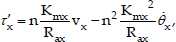
From (33)-(36), we know that the dynamic equations in the x and y-axes are identical. Also, the actuation mechanisms driving the tilts of the plate in the x and y-axes are identical. In the following, only the ball and beam system and the actuation mechanism in the x-axis will be discussed. The inclination of the plate is driven by a four-bar linkage as shown in Figure 9, where τ‘_x is the torque generated by the motor, and τ_x is the torque exerted on the plate. Based on the force analysis, we have

Figure 9.

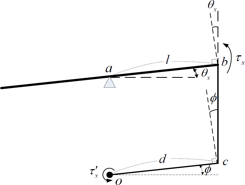
Connections of the linkages and plate.

${\tau }_x=\frac{l}{d}{\tau }_x^{\prime }\cos {\theta }_x\cos \varphi .$

(37)

We assume that the angles of θ_x and ϕ are small enough that lsin θ_x = dsinϕ can be simplified as

$l{\theta }_x\cong d\varphi .$

Since l = d, we have

${\theta }_x\cong \varphi .$

(38)

Note that θ_x is not directly measurable. However, for feedback control, θ_x can be approximated by the measurement of the angular displacement of the motor shaft. Moreover, (37) can be rewritten as

${\tau }_x\cong {\tau }_x^{\prime }{\cos }^2{\theta }_x.$

(39)

A voltage signal, which is generated according to a control law as designed below, is supplied to an amplifier, which drives the permanent-magnet dc motor to control the L-shaped linkage. Since the electrical time constant of a dc motor is usually much smaller than the mechanical time constant, and the value of the viscous friction coefficient is negligible, the following reduced-order model [24] of the dc motor is adopted:

${\tau }_x^{\prime }=n\frac{K_{mx}}{R_{ax}}{v}_x-n^2\frac{K_{mx}{}^2}{R_{ax}}{\stackrel{.}{\theta }}_x,$

(40)

where v_x is the control voltage, K_mx is the motor constant, is the armature resistance, and n is the gear ratio. In this study, the value of n is chosen as 8.

The state vector is defined as

${\left[x_1 x_2 x_3 x_4\right]}^{\mathrm{T}}={\left[y \stackrel{.}{y} {\theta }_x {\stackrel{.}{\theta }}_x\right]}^{\mathrm{T}}.$

(41)

From (34), (35), (39), and (40), the state space equation of the system on the basis of (41) can be written as:

$\left[\begin{array}{c}{\stackrel{.}{x}}_1\\ {\stackrel{.}{x}}_2\\ {\stackrel{.}{x}}_3\\ {\stackrel{.}{x}}_4\end{array}\right]=\left[\begin{array}{c}{x}_2\\ E(x_1{x}_4^2-g\sin x_3)\\ x_4\\ 0\end{array}\right]+\left[\begin{array}{c}0\\ 0\\ 0\\ 1\end{array}\right]u_x,$

(42)

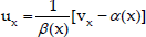
where u_x is the new control input, which is given by

$\begin{array}{l}{u}_x=\frac{1}{J_{px}+J_b+m{x}_1{}^2}[(8\frac{K_{mx}}{R_{ax}}{v}_x-64\frac{K_{mx}^2}{R_{ax}}{x}_4){\cos }^2{x}_3\\ -2m{x}_1{x}_2{x}_4+mg{x}_1\cos x_3+mgR\sin x_3]\end{array}$

(43)

and

$E=\frac{m}{m+\frac{J_b}{R^2}}.$

The state space equation (42) is used for later control design. The physical parameters of the system are listed in Table 2.

Table 2.

Physical Parameters

Description	Symbol	Value	Unit
Mass of the plate	m	0.56	kg
Radius of the ball	R	0.011	m
Moment of inertia of the ball	Jb	2.4210−6	kg.m2
Moment of inertia of the plate about the x-axis	Jpx	7.46610−3	kg.m2
Moment of inertia of the plate about the y-axis	Jpy	7.46610−3	kg.m2
Moment of inertia of the plate about the z-axis	Jpz	14.93310−3	kg.m2
Gravitational acceleration	g	9.8	m.sec−2
Motor constant	Kmx	0.045	N.m/A
Motor armature resistance	Rax	8.95	Ω

Based on the perspective projection (1), the machine vision system measures the position of the ball relative to the space-fixed coordinate oXYZ. To determine the actual position of the ball relative to the plate-fixed coordinate oxyz, we consider the coordinates of the centre of the ball measured by the machine vision system and the actual coordinates relative to the plate-fixed coordinate as shown in Figure 10.

Figure 10.

Coordinates of the centre of the ball measured by the machine vision system and the actual coordinates relative to the plate-fixed coordinate.

Here, the point A with coordinates [0, 0, d_c]^T relative to the space-fixed coordinate is the origin of the camera frame. The point B with coordinates [X, Y, R]^T relative to the space-fixed coordinate is the centre of the ball measured by the machine vision system. The point C with coordinates [x, y, R]^T relative to the plate-fixed coordinate is the actual centre of the ball. The coordinates of the point A relative to the plate-fixed coordinate are denote by [a_x, a_y, a_z]^T, which can be obtained using (11):

$\left[\begin{array}{l}{a}_x\\ a_y\\ a_z\end{array}\right]={\hspace{0.17em}}^{P}R{}_F\left[\begin{array}{l}0\\ 0\\ d_c\end{array}\right].$

(44)

The coordinates of the point B relative to the plate-fixed coordinate are denoted by [b_x,b_y,b_z]^T, which can be obtained by

$\left[\begin{array}{l}{b}_x\\ b_y\\ b_z\end{array}\right]={\hspace{0.17em}}^{P}R{}_F\left[\begin{array}{l}X\\ Y\\ R\end{array}\right].$

(45)

Based on the perspective projection, the points A, B, C must be collinear. Thus, we have

$\frac{x-a_x}{b_x}=\frac{y-a_y}{b_y}=\frac{R-a_z}{b_z}.$

(46)

From (46), the centre of the ball on the x-y plane of the plate-fixed coordinate is given by

$x=a_x+\frac{R-a_z}{b_z}{b}_x,$

(47)

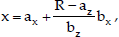
and

$y=a_y+\frac{R-a_z}{b_z}{b}_y.$

(48)

5. Tracking Control Design Based on Approximate Input-Output Feedback Linearization

This far, we have discussed the ball and plate system simplified into two decoupled ball and beam systems. In this section, for each decoupled ball and beam system we use an approximate input-output feedback linearization technique to design a tracking control law.

Consider a single-input single-output system of the form

$\stackrel{.}{x}=f(x)+g(x)u,$

(49)

$y_o=h(x),$

(50)

where x ∈ Rⁿ,u and y_o ∈ R, f and g are smooth vector fields on Rⁿ, and h: Rⁿ → R is a smooth scalar function. We assume that x = 0 is an equilibrium point of the system. The derivative of h(x) along vector field f(x) is expressed by the Lie derivative $L_{f}h(x)=\frac{\partial h}{\partial x}f(x),$ , while $L_f^{2}h(x)$ stands for L_f(L_fh)(x), and $L_f^{k}h(x)$ denotes $L_f(L_f^{k-1}h)(x).$ . Note that $L_g{L}_{f}h(x)=\frac{\partial L_{f}h(x)}{\partial x}g(x),$ , while $L_g{L}_f^{k}h(x)$ stands for $L_g{L}_f(L_f^{k-1}h)(x)$ , and so on. We take subsequent derivatives of the output until, say at γ, the control appears, and we obtain

$\begin{array}{l}{\stackrel{.}{y}}_o=L_{f}h(x),\\ {\stackrel{..}{y}}_o=L_f^{2}h(x),\\ \hspace{1em}⋮\\ y_o{}^{(\gamma )}=L_f^{\gamma }h(x)+L_g{L}_f^{\gamma -1}h(x)u.\end{array}$

(51)

The system of (49) and (50) is said to have the relative degree γ, which is well-defined in an open neighbourhood U of the origin if for $x\in U$ $L_g{L}_f^{i}h(x)=0$ with i = 0, 1, …, γ − 2, and $L_g{L}_f^{\gamma -1}h(x)\ne 0$ . Then, the feedback control law $u=\frac{-L_f^{\gamma }h(x)+v}{L_g{L}_f^{\gamma -1}h(x)}$ achieves the input-output linearization from v to y_o.

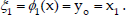
In [20], it was shown that the relative degree of the ball and beam system is not well defined at certain locations, and this system violates the involutivity conditions of feedback linearization. Therefore, neither exact input-output feedback linearization nor full-state feedback linearization is applicable to this particular system. Alternatively, the approximate input-output feedback linearization proposed in [20] provides a method to find a set of coordinate transforms ξ_i = ϕ_i(x), i = 1,…,γ, that approximate the output and its subsequent derivatives. The idea of approximate input-output feedback linearization is to construct the coordinate transform in the usual fashion as in the exact input-output feedback linearization by neglecting the second or higher order terms in the approximate output and its subsequent derivatives. We consider the ball and beam system of (42) with the output y_o=h(x) = x₁. To proceed with approximate input-output feedback linearization, a smooth function ϕ₁(x) is chosen to approximate the output

${\xi }_1={\varphi }_1(x)=y_o=x_1.$

(52)

Then, we obtain

$\begin{array}{l}{\stackrel{.}{\xi }}_1={\stackrel{.}{y}}_o=\underset{{\varphi }_2(x)}{\underbrace{x_2}},\\ {\stackrel{.}{\xi }}_2={\stackrel{..}{y}}_o=\underset{{\varphi }_3(x)}{\underbrace{E{x}_1{x}_4^2-Eg\sin x_3}},\\ {\stackrel{.}{\xi }}_3={\stackrel{⃛}{y}}_o=\underset{{\varphi }_4(x)}{\underbrace{E{x}_2{x}_4^2-Eg{x}_4\cos x_3}}+\underset{\begin{array}{l}\text{disgard this }\\ \text{high order term}\end{array}}{\underbrace{2E{x}_1{x}_4{u}_x}},\\ {\stackrel{.}{\xi }}_4=y_o{}^{(4)}=E^2{x}_1{x}_4^4+E(1-E)x_4^2\sin x_3\\ +(-Eg\cos x_3+2E{x}_2{x}_4)u_x.\end{array}$

(53)

The term of 2Ex₁x₄u_x in ${\stackrel{⃛}{y}}_o$ is discarded, and then y_o⁽⁴⁾ is obtained by taking the derivative of ϕ₄(x). By neglecting the term 2Ex₁x₄u_x and using the coordinate transformation

$\begin{array}{l}{\xi }_1={\varphi }_1(x)=x_1,\\ {\xi }_2={\varphi }_2(x)=x_2,\\ {\xi }_3={\varphi }_3(x)=E{x}_1{x}_4^2-Eg\sin x_3,\\ {\xi }_4={\varphi }_4(x)=-Eg{x}_4\cos x_3+E{x}_2{x}_4^2,\end{array}$

(54)

we obtain a feedback linearizable system given by

$\begin{array}{l}{\stackrel{.}{\xi }}_1={\xi }_2,\\ {\stackrel{.}{\xi }}_2={\xi }_3,\\ {\stackrel{.}{\xi }}_3={\xi }_4,\\ {\stackrel{.}{\xi }}_4=\alpha (x)+\beta (x)u_x,\end{array}$

(55)

where $\alpha (x)=E^2{x}_1{x}_4^4+E(1-E)x_4^2\sin x_3 ,$ , and β(x) = –Egcosx₃ +2Ex₂x₄. Thus, the feedback control law

$u_x=\frac{1}{\beta (x)}[v_x-\alpha (x)]$

(56)

approximately linearizes the ball and beam system of (42) with the output y_o = h(x) = x₁ from v to y_o up to the terms of O(x,u_x)². Here, a scalar function δ(x) is said to be O(x)ⁿ if $\underset{\Vert x\Vert \to 0}{\lim }\frac{\left|\delta (x)\right|}{{\Vert x\Vert }^n}$ exists and is not zero. Note that there exists a neighbourhood of the equilibrium, in which β(x) ≠ 0. Since the control objective is to make the output y_o track a desired trajectory y_d, approximate tracking can be obtained by choosing $u_x=\frac{1}{\beta (x)}[v_x-\alpha (x)]$ with

$\begin{array}{l}{v}_x=y_{dx}^{(4)}+K_3({\stackrel{⃛}{y}}_{dx}-{\xi }_4)+K_2({\stackrel{..}{y}}_{dx}-{\xi }_3),\\ +K_1({\stackrel{.}{y}}_{dx}-{\xi }_2)+K_0(y_{dx}-{\xi }_1)\end{array}$

(57)

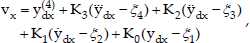
where K_i are chosen so that s⁴+K₃s³+K₂s² + K₁s+K₀ is a Hurwitz polynomial.

To analyse the tracking error and stability of the closed-loop system, we define the state vector and control input in the x and y-axes thus:

$\begin{array}{l}{x}_p^{\mathrm{T}}={\left[\begin{array}{cccccccc}{x}_1& x_2& x_3& x_4& x_5& x_6& x_7& x_8\end{array}\right]}^{\mathrm{T}}\\ ={\left[\begin{array}{cccccccc}y& \stackrel{.}{y}& {\theta }_x& {\stackrel{.}{\theta }}_x& x& \stackrel{.}{x}& {\theta }_y& {\stackrel{.}{\theta }}_y\end{array}\right]}^{\mathrm{T}},\\ u^{\mathrm{T}}={\left[\begin{array}{cc}{u}_x& u_y\end{array}\right]}^{\mathrm{T}}\end{array}$

(58)

Then, the ball and plate system can be written as two decoupled ball and beam systems with higher order coupling terms as follows:

$\begin{array}{l}\left[\begin{array}{c}{\stackrel{.}{x}}_1\\ {\stackrel{.}{x}}_2\\ {\stackrel{.}{x}}_3\\ {\stackrel{.}{x}}_4\\ {\stackrel{.}{x}}_5\\ {\stackrel{.}{x}}_6\\ {\stackrel{.}{x}}_7\\ {\stackrel{.}{x}}_8\end{array}\right]=\left[\begin{array}{c}{x}_2\\ E(x_1{x}_4^2-g\sin x_3)\\ x_4\\ 0\\ x_6\\ E(x_5{x}_8^2-g\sin x_7)\\ x_8\\ 0\end{array}\right]+\left[\begin{array}{cc}0& 0\\ 0& 0\\ 0& 0\\ 1& 0\\ 0& 0\\ 0& 0\\ 0& 0\\ 0& 1\end{array}\right]u+\mathrm{\Delta }f(x_p,u),\\ \left[\begin{array}{c}{y}_{ox}\\ y_{oy}\end{array}\right]=\left[\begin{array}{c}{x}_1\\ x_5\end{array}\right],\end{array}$

(59)

where Δf(x_p,u) are the higher order coupling terms. y_ox and y_oy are the outputs in the x and y-axes, respectively. Using the coordinate transforms (54) and feedback control law (56), the approximate input-output feedback linearization for the system (59) is given by

$\begin{array}{l}\left[\begin{array}{c}{\stackrel{.}{\xi }}_1\\ {\stackrel{.}{\xi }}_2\\ {\stackrel{.}{\xi }}_3\\ {\stackrel{.}{\xi }}_4\\ {\stackrel{.}{\xi }}_5\\ {\stackrel{.}{\xi }}_6\\ {\stackrel{.}{\xi }}_7\\ {\stackrel{.}{\xi }}_8\end{array}\right]=\left[\begin{array}{cccccccc}0& 1& 0& 0& 0& 0& 0& 0\\ 0& 0& 1& 0& 0& 0& 0& 0\\ 0& 0& 0& 1& 0& 0& 0& 0\\ 0& 0& 0& 0& 0& 0& 0& 0\\ 0& 0& 0& 0& 0& 1& 0& 0\\ 0& 0& 0& 0& 0& 0& 1& 0\\ 0& 0& 0& 0& 0& 0& 0& 1\\ 0& 0& 0& 0& 0& 0& 0& 0\end{array}\right]\left[\begin{array}{c}{\xi }_1\\ {\xi }_2\\ {\xi }_3\\ {\xi }_4\\ {\xi }_5\\ {\xi }_6\\ {\xi }_7\\ {\xi }_8\end{array}\right]+\left[\begin{array}{cc}0& 0\\ 0& 0\\ 0& 0\\ 1& 0\\ 0& 0\\ 0& 0\\ 0& 0\\ 0& 1\end{array}\right]\left[\begin{array}{c}{v}_x\\ v_y\end{array}\right]+\psi (x_p,u),\\ \left[\begin{array}{c}{y}_{ox}\\ y_{oy}\end{array}\right]=\left[\begin{array}{c}{\xi }_1\\ {\xi }_5\end{array}\right],\end{array}$

(60)

where ψ(x_p,u) are the summation of the higher order coupling terms Δf(x_p,u) and the approximation errors. We define the tracking error vector e as

$\left[\begin{array}{c}{e}_1\\ e_2\\ e_3\\ e_4\\ e_5\\ e_6\\ e_7\\ e_8\end{array}\right]=\left[\begin{array}{c}{\xi }_1\\ {\xi }_2\\ {\xi }_3\\ {\xi }_4\\ {\xi }_5\\ {\xi }_6\\ {\xi }_7\\ {\xi }_8\end{array}\right]-\left[\begin{array}{c}{y}_{dx}\\ {\stackrel{.}{y}}_{dx}\\ {\stackrel{..}{y}}_{dx}\\ {\stackrel{⃛}{y}}_{dx}\\ y_{dy}\\ {\stackrel{.}{y}}_{dy}\\ {\stackrel{..}{y}}_{dy}\\ {\stackrel{⃛}{y}}_{dy}\end{array}\right].$

(61)

With the stable tracking control law (57), the closed-loop system can be then written as

$\stackrel{.}{e}=Ae+\psi \left(x_p,u(x_p,y_d)\right),$

(62)

where $y_d^{\mathrm{T}}=\left[\begin{array}{cccccccc}{y}_{dx}& {\stackrel{.}{y}}_{dx}& {\stackrel{..}{y}}_{dx}& {\stackrel{⃛}{y}}_{dx}& y_{dy}& {\stackrel{.}{y}}_{dy}& {\stackrel{..}{y}}_{dy}& {\stackrel{⃛}{y}}_{dy}\end{array}\right]$ and A is an 8×8 matrix with all its eigenvalues in the open left-half complex plane. Since ψ(x_p,u(x _p ,y_d)) is a so-called uniformly higher order function [20], there exist ∈ > 0, d > 0, and a function K _∈ , which is a monotonically increasing function of ∈, such that

$\Vert \psi \left(x_p,u(x_p,y_d)\right)\Vert \le \epsilon K_{\epsilon }\left(\Vert e\Vert +d\right)$

(63)

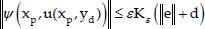
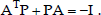
for x_p ∈ U _∈ ⊂ R⁸ and ‖y_d‖ ≤ d. Since A is a Hurwitz matrix, there exists a positive definite matrix P such that

$A^{\mathrm{T}}P+PA=-I.$

(64)

Consider the Lyapunov candidate function for the error system (62):

$V=e^{\mathrm{T}}Pe .$

(65)

The derivative of V along the trajectories of (62) is given by

$\begin{array}{l}\stackrel{.}{V}=-{\Vert e\Vert }^2+2e^{T}P\psi \left(x_p,u(x_p,y_d)\right)\hfill \\ \le \begin{array}{cc}-{\Vert e\Vert }^2+\epsilon K_{\epsilon }\mu \Vert e\Vert \left(\Vert e\Vert +d\right)\hfill & \text{(for some}\end{array} \mu >0)\hfill \\ \le -\left(\frac{1}{2}-\epsilon K_{\epsilon }\mu \right){\Vert e\Vert }^2-{\left(\frac{\Vert e\Vert }{\sqrt{2}}-\frac{1}{\sqrt{2}}\epsilon k_{\epsilon }\mu d\right)}^2+\frac{1}{2}{\left(\epsilon k_{\epsilon }\mu d\right)}^2\hfill \\ \le -\left(\frac{1}{2}-\epsilon K_{\epsilon }\mu \right){\Vert e\Vert }^2+\frac{1}{2}{\left(\epsilon k_{\epsilon }\mu d\right)}^2\hfill \end{array}$

(66)

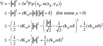
Then, for all $\epsilon \le \frac{1}{4K_{\epsilon }\mu }$ , it follows that

$\stackrel{.}{V}\le -\frac{{\Vert e\Vert }^2}{4}+\frac{{(\epsilon k_{\epsilon }\mu d)}^2}{2}.$

(67)

Therefore, V̇ < 0 whenever ‖e‖ is large, which implies that ‖e‖ and, hence, the states of the closed-loop system are bounded. Moreover, for a sufficiently small reference command ‖y_d‖ and appropriate initial conditions, we can conclude that the tracking error is of order O(∈).

6. Simulation and Experimental Results

To measure the performance of the designed control law, the control system was simulated in MATLAB/Simulink using the parameters in Table 2. The control gains of (57) were chosen to be [K₃, K₂, K₁, K₀]=[8.7788, 145.6124, 799.0362, 1998.3245]. The simulation of circular trajectory tracking was conducted. The ball was commanded to follow a circular trajectory of radius 0.08 m, centred at the origin with a constant angular speed of 0.75 rad/sec. The corresponding trajectory references of each axis are y_dx =0.08sin(0.75t) and y_dy = 0.08cos(0.75t). The initial conditions were set to x = 0 m, y = 0 m, θ_x = 0 rad, θ _y = 0 rad, ẋ = 0 m/sec, ẏ = 0 m/sec, $\stackrel{.}{y}=0 \text{m/sec}$ rad/sec, and θ_y = 0 rad/sec. The simulation results of the position responses of the ball, the angular position responses of the inclining plate, the control voltages, position errors, and the trajectory of the ball are shown in Figure 11(a), (b), (c), (d) and (e), respectively. As shown in Figure 11(a) and (e), the ball converges towards the desired trajectory in 2 seconds with a starting point at the origin. The position errors are shown in Figure 11(d). This confirms that the static error in tracking a commanded trajectory is very small, as mentioned in Section 5. The operating range of the control voltage, which is ±20 V, is constrained by the motor driver.

Figure 11 (a-1)

Comparison of simulation results (dash-dot line) of the position responses of the ball and tracking command (solid line) in the x-axis.

Figure 11 (a-2)

Comparison of simulation results (dash-dot line) of the position responses of the ball and tracking command (solid line) in the y-axis.

Figure 11 (b-1)

Simulation result of the angular position response of the inclining plate in the x-axis.

Figure 11 (b-2)

Simulation result of the angular position response of the inclining plate in the y-axis.

Figure 11 (c-1)

Simulation result of the control voltage v_x.

Figure 11 (c-2)

Simulation result of the control voltage v_y.

Figure 11 (d)

Simulation results of the position error of the x-axis (dash-dot line) and position error of the y-axis (solid line).

Figure 11 (e)

Comparison of the simulation result (dash-dot line) of the trajectory of the ball and commanded trajectory (solid line).

Figure 11(c) shows that the control voltages did not saturate in the simulation for the chosen initial conditions and trajectory references.

For further validation, the designed control law and image processing algorithms were implemented and tested on the experimental setup, as shown in Figure 1. The image processing algorithms were implemented on the FPGA board in VHDL. The designed controller was implemented on the DSP system in C. The camera in the proposed system operated at 150 frames/sec. Thus, the sampling frequency of the system was set to 150 Hz.

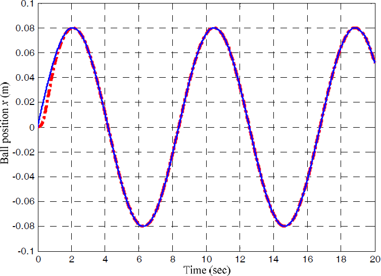
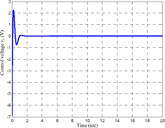
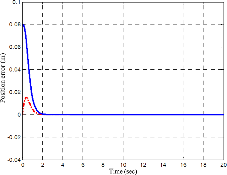
The trajectory tracking experiment was conducted with the same initial conditions and controller parameters as in the simulation. The experimental results of the position responses of the ball, the angular position responses of the inclining plate, the control voltages, position errors, and the trajectory of the ball are shown in Figure 12(a), (b), (c), (d), and (e), respectively. As shown in Figure 12(a) and (e), the ball converged towards the desired trajectory in 1.9 seconds with a starting point at the origin. In Figure 12(d) it can be observed that the static position error in the x-axis is within a range from −0.0094 m to 0.0049 m, while the static position error in the y-axis is within a range from −0.0080 m to 0.0091 m. It also shows a good agreement between simulation results and experimental results. The mismatch and amplitude oscillations between simulation and experimental results are possibly caused by approximation errors in control design, disturbances, and unmodelled hardware effects such as friction, ball slipping, plate unevenness, illumination variation, low resolution of the camera (352×288 pixels), etc. As shown in the analysis of tracking error and stability, one can choose a small reference command and initial conditions with a small initial tracking error to improve tracking performance.

Figure 12 (a-1)

Comparison of experimental result (dash-dot line) of the position response of the ball and tracking commands (solid line) in the x-axis.

Figure 12 (a-2)

Comparison of experimental result (dash-dot line) of the position response of the ball and tracking commands (solid line) in the y-axis.

Figure 12 (b-1)

Experimental result of theangular position response of the inclining plate in the x-axis.

Figure 12 (b-2)

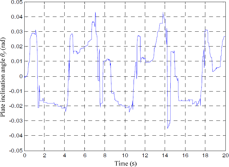
Experimental result of the angular position response of the inclining plate in the y-axis.

Figure 12 (c-1)

Experimental result of the control voltage v_x.

Figure 12 (c-2)

Experimental result of the control voltage v_y.

Figure 12 (d)

Experimental results of the position error of the x-axis (dash-dot line) and position error of the y-axis (solid line).

Figure 12 (e)

Comparison of the experimental result (dot line) of the trajectory of the ball and commanded trajectory (solid line).

For a camera with a low frame rate, visual servoing can result in performance degradation or even closed-loop instability. The obtained controller was discretized by the Tustin's method. The control system was then simulated in MATLAB/Simulink. From the simulation shown in Figure 13, we found that the closed-loop system becomes unstable for trajectory tracking when the sampling time is greater than 43 ms (23.26 Hz). The tested system cannot be stabilized if the frame rate is below 31 frames/sec. This is the reason this system requires a fast camera. A video clip demonstrating the performance of the developed system is available at http://lab.es.ncku.edu.tw/csplab/ball&plate-wmv.htm. The video shows that the system performs well even with different initial conditions and disturbance.

Figure 13.

System becomes unstable when system performs trajectory tracking with a sampling time of 43 ms.

7. Conclusions

Visual servoing tracking control for a ball and plate system was designed, implemented, and validated. The experimental setup, system modelling and implementation of the machine vision system were described in detail. The main contribution of this paper is twofold. First, the complete system model was derived for system simulation and analysis. Approximate input-output feedback linearization was used to design the control law for trajectory tracking. Second, an FPGA implementation was used to carry out image processing algorithms to achieve real-time constraints.

The performance of the designed control system was investigated via simulated and experimental responses providing comparisons and the validation of controller design and system modelling. Both simulation and experimental results showed that the designed system had good performance. This experimental setup can serve as a test bed for nonlinear control schemes as well as supporting laboratory practice.