Sage Journals: Discover world-class research

Abstract

We consider a path planning problem where a team of Unmanned Vehicles (UVs) is required to visit a given set of targets. The UVs are assumed to carry different sensors, and as a result, there are vehicle-target constraints that require each UV to visit a distinct subset of targets. The objective of the path planning problem is to find a path for each UV such that each target is visited at least once by some vehicle, the vehicle-target constraints are satisfied and the total distance travelled by the vehicles is a minimum. This path planning problem is a generalization of the Hamiltonian path problem and is NP-Hard. We develop a primal-dual heuristic and incorporate the heuristic in a Lagrangian relaxation procedure to find good, feasible solutions and lower bounds for the path planning problem. Computational results show that solutions whose costs are on an average within 14% of the optimum can be obtained relatively quickly for the path planning problem involving five UVs and 40 targets.

Keywords

Unmanned Vehicle Hamiltonian Path Problem Primal-Dual Method Lagrangian Relaxation Subgradient Algorithm

1. Introduction

Surveillance applications involving Unmanned Vehicles (UVs) require UVs with different capabilities to gather information about a set of targets [3]. Information is often gathered using the sensors on-board the UVs while visiting the targets. In these missions, it is possible that UVs carry different sensors due to resource constraints. As a result, there may be vehicle-target constraints that require a specific vehicle to visit a subset of targets. We consider a basic path planning problem that commonly arises in these surveillance applications: Given a set of vehicles and targets, the objective of this problem is to find a path for each vehicle such that each target is visited at least once by some vehicle, the vehicle-target constraints are satisfied and the sum of the distances travelled by all the vehicles is a minimum.

The difficulty with solving this path planning problem for the UVs is mainly combinatorial. While the motion constraints of the UV complicate the problem, they are not a source of difficulty as long as the trajectory of least distance to go from an origin to a destination can be efficiently computed; it does not matter whether the vehicle is modelled as a double integrator or a Dubins [9] or a Reeds-Shepp [17] vehicle. To illustrate this point about the combinatorial nature of the problem, consider the path planning problem for just one UV modelled as a Dubins vehicle [9]. If the “optimal” heading angles were to be specified at each and every target, the problem of finding the optimal sequence of targets to be visited reduces to the notoriously hard Hamiltonian Path Problem (HPP), which is known to be NP-Hard in the literature [1]. However, if the “optimal” sequence were to be given, the “optimal” heading angles can be found using dynamic programming and can be determined arbitrarily accurately as a shortest path problem in a network [21], a problem for which efficient algorithms exist [7].

For the above reasons, we assume that the heading angle at which a vehicle must visit each target is known. We also assume that the cost of travelling for a UV from target A at an initial heading angle (ψ_A) to target B at a final heading angle (ψ_B) can be computed and is known. Therefore, finding a sequence of targets to visit for a vehicle is equivalent to specifying the path for the vehicle. Using these assumptions, our problem can be viewed as a multiple depot, multiple vehicle, asymmetric¹ HPP with additional vehicle-target constraints. In the context of UVs, we are not aware of algorithms that directly address this problem in the literature. However, there are approximation algorithms and heuristics for similar problems. For example, Doshi et al. [8] present heuristics and an approximation algorithm for a 2-depot, symmetric HPP. Approximation algorithms are presented for a multiple depot, symmetric HPP in [20]. A heuristic based on a transformation method is also presented for a multiple depot, asymmetric, heterogeneous TSP by Oberlin et al. in [15]. The combinatorial problem considered in this article is a special case of more difficult vehicle routing problems for which heuristics are presented in [4],[6],[5],[16]. In this article, we develop a primal-dual heuristic and incorporate the heuristic in a Lagrangian relaxation procedure to find good, feasible solutions and lower bounds for the path planning problem. Computational results show that solutions whose costs are within 14% of the optimum can be obtained relatively quickly for the path planning problem involving five UVs and 40 targets.

2. Problem Statement

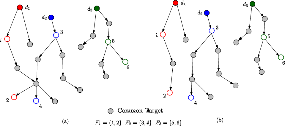
Let there be n vehicles initially located at distinct depots denoted by d₁, d₂, …, d_n and let D:={d₁, …, d_n (Refer to Figure 1). Let T denote the set of targets that needs to be visited by the vehicles. Let F_k ⊆ T represent the subset of targets that must be visited by the vehicle initially located at depot d_k. C:=T\Uⁿ_i=1 F_k denotes the subset of all the targets that can be visited by any vehicle. We assume $F_{k} \cap F_{k^{'}} = Ø$ for all $k, k^{'} \in {1, \dots, n}, k \neq k^{'}$ . The Multiple Vehicle Problem (MVP) is formulated on the complete directed graph G = (V, E), where V = D ∪ T and E represents the set of all the edges between any two distinct vertices in V. For any two distinct vertices i and j, the edge directed from vertex i to vertex j is denoted by (i, j). Let c_ij represent the cost of travelling from vertex i to vertex j for any vehicle. The objective of the problem is to find a path for each vehicle such that

the paths for the vehicles start at their respective depots,

each target in F_k is visited at least once by the vehicle located at depot d_k,

each common target is visited at least once by some vehicle, and,

the total cost of travelling the edges in all the paths is a minimum.

An illustration of a feasible solution to this MVP is shown in Figure 1.

Figure 1.

A solution to the path planning problem. F₁, F₂ and F₃ denote the subsets of targets that need to be visited by the vehicles at depots d₁, d₂ and d₃ respectively.

3. Problem Formulation

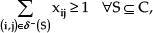
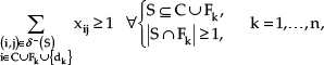
In this section, we formulate the problem as an integer program. Let x_ij be the binary decision variable that represents the presence of edge (i, j) in the solution; that is, x_ij is equal to 1 if a vehicle is travelling from vertexi to vertex j and is equal to 0 otherwise. For any S ⊂ V, let ™⁻(S) ⊆ E denote the set of all the edges directed into S, i.e, for any (i, j) ∈ ™⁻(S),i ∈ V\S and j ∈ S. Similarly, let ™⁺(S) represent the set of all the edges directed out of S, that is, for any (i, j) ∈ ™⁺(S),i ∈ S and j ∈ V\S. The MVP is formulated as an integer program as follows:

f^{*} = \min \sum_{(i, j) \in E} c_{i j} x_{i j}

subject to

\sum_{i \in V, i \neq j} x_{i j} \leq 1 \forall j \in V,

(1)

\sum_{j \in V, i \neq j} x_{i j} \leq 1 \forall i \in V,

(2)

\sum_{(i, j) \in δ^{-} (S)} x_{i j} \geq 1 \forall S \subseteq C,

(3)

\sum_{\begin{array}{l} (i, j) \in δ^{-} (S) \\ i \in C \cup F_{k} \cup {d_{k}} \end{array}} x_{i j} \geq 1 \forall {\begin{matrix} S \subseteq C \cup F_{k}, \\ | S \cap F_{k} | \geq 1, \end{matrix} k = 1, \dots, n,

(4)

x_{i j} = {0, 1} \forall (i, j) \in E .

(5)

Equations (1) and (2) require that the in-degree and out-degree of each vertex be at most equal to one. Constraints (3), (4) ensure that each common target is connected to at least one depot and each functionally heterogeneous target is connected to its respective depot. Specifically, equation (3) requires that there must be at least one incoming edge to every subset of common targets. Similarly, equation (4), requires that there must be at least one suitable edge directed into every subset consisting of common targets and at least one target from F_k for any k. For example, if the subset S consists of a target from F₁ and some common targets, then a suitable incoming edge into S can be directed either from the depot d₁, or from a common target, or from a target in F₁ but not in S.

4. Lagrangian Relaxation of the MVP

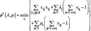
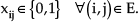
A Lagrangian relaxation for the MVP can be obtained by removing the constraints that complicate the formulation in (1)-–(4), and penalizing them in the objective if they are violated. This idea was first successfully applied to a single vehicle routing problem by Held and Karp in [13]. Suppose the degree constraints in (1) and (2) are relaxed, and let λ_i and µ_i be the penalty variables corresponding to the degree constraint of vertex i in (1) and (2) respectively. Let λ denote the vector (λ₁,…,λ_|V|), and μ represent (μ₁,…,μ_|V|). Then, for an λ, µ≥ 0, we obtain a Lagrangian relaxation as follows:

ϕ^{*} (λ, μ) = \min_{x} {\begin{cases} \sum_{(i, j) \in E} c_{i j} x_{i j} + \sum_{j \in V} λ_{j} (\sum_{i \in V, i \neq j} x_{i j} - 1) \\ + \sum_{i \in V} μ_{i} (\sum_{j \in V, i \neq j} x_{i j} - 1) \end{cases}}

(6)

subject to

\sum_{(i, j) \in δ^{-} (S)} x_{i j} \geq 1 \forall S \subseteq C,

(7)

\sum_{\begin{array}{l} (i, j) \in δ^{-} (S) \\ i \in C \cup F_{k} \cup {d_{k}} \end{array}} x_{i j} \geq 1 \forall {\begin{matrix} S \subseteq C \cup F_{k}, \\ | S \cap F_{k} | \geq 1, \end{matrix} k = 1, \dots, n,

(8)

x_{i j} \in {0, 1} \forall (i, j) \in E .

(9)

The objective of the above relaxation can be re-written as follows:

\begin{array}{l} φ (λ, μ, x) = \sum_{(i, j) \in E} c_{i j} x_{i j} + \sum_{j \in V} λ_{j} (\sum_{i \in V, i \neq j} x_{i j} - 1) + \sum_{i \in V} μ_{i} (\sum_{j \in V, i \neq j} x_{i j} - 1), \\ = \sum_{(i, j) \in E} (c_{i j} + λ_{j} + μ_{i}) x_{i j} - \sum_{j \in V} λ_{j} - \sum_{i \in V} μ_{i} \\ = \sum_{(i, j) \in E} {\hat{c}}_{i j} x_{i j} - K (λ, μ), \end{array}

where the modified cost ĉ _ij = c _ij + λ_j + μ _i , and K(λ,μ) = Σ_j∈Vλ_j + Σ_i∈Vμ_i.

It is well known in the literature [11] that the optimal cost of a Lagrangian relaxation always provides a lower bound for the corresponding integer programming problem. In relation to the MVP, this result implies that φ*(λ,µ) ≤f*for any λ,µ ≥0 where f* denotes the optimal cost of the MVP. One can then obtain the best or the tightest lower bound for the MVP by solving the following problem: max_λ,µ≥0 φ* (λ,µ). This problem of maximizing the lower bound will be referred to as the Lagrangian dual problem in this article.

Suppose F denotes the set of all the solutions (a solution consists of a forest of edges; refer to Figure 2 for an illustration) that satisfy the constraints in (7)–(9). Then, the Lagrangian dual problem can be stated as

\begin{array}{l} \max_{λ, µ \geq 0} φ^{*} (λ, µ) = \max_{λ, µ \geq 0} \min_{x \in F} \\ (\sum_{(} {_{i, j}}_{) \in x} (c_{i j} + λ_{j} + µ_{i}) x_{i j} - \sum_{j \in V} λ_{j} - \sum_{i \in V} µ_{i}) . \end{array}

Even though the Lagrangian dual problem is a non-smooth optimization problem, note that the objective φ* (λ,µ) is a concave function of the penalty variables in λ and µ. Therefore, one can use a subgradient algorithm as in [13],[18] to solve the Lagrangian dual problem.

A crucial part of solving the Lagrangian dual problem involves solving the minimization problem in (6)–(9). This minimization problem aims to find a forest of edges such that

there is a directed path from a depot to each of the common targets,

there is a directed path from the depot d_k to each of the targets in F_k for k =1,…,n, and,

the sum of the cost of the edges in this forest is a minimum.

If there is only one vehicle and there are no vehicle-target constraints, this minimization problem reduces to solving a directed spanning tree which can be computed in polynomial time. If there are multiple vehicles with additional vehicle-target constraints, it is not yet known if this minimization problem can be solved in polynomial time. However, we circumvent this difficulty by developing a primal-dual heuristic which provides a good lower bound and a feasible solution to the minimization problem. We use this feasible solution (a forest) to partition the common targets such that each common target is assigned to some vehicle. Once a subset of targets is assigned to a vehicle, we use the Lin-Kernighan Heuristic (LKH) to find a path for the vehicle. Using the above procedure, given the penalty variables in λ and µ, one can find a lower bound and a feasible solution for the MVP. In the next section, we discuss the primal-dual heuristic. Later, we present the subgradient algorithm that uses this primal-dual heuristic to solve the Lagrangian dual problem.

Figure 2.

Feasible solutions for the Lagrangian relaxation. Notice that in (a) some common targets are connected to depots d₁ and d₂, whereas each common target is connected to exactly one depot in (b).

5. Primal Dual Heuristic for solving the Lagrangian Relaxation

Given the penalty variables in λ and µ, consider the basic minimization problem in the Lagrangian relaxation:

\begin{array}{c} \min \sum_{(i, j) \in E} {\hat{c}}_{i j} x_{i j} \\ \sum_{(i, j) \in δ^{-} (S)} x_{i j} \geq 1 \forall S \subseteq C, \end{array}

(10)

\sum_{\begin{array}{l} (i, j) \in δ^{-} (S) \\ i \in C \cup F_{k} \cup {d_{k}} \end{array}} x_{i j} \geq 1 \forall {\begin{matrix} S \subseteq C \cup F_{k}, \\ | S \cap F_{k} | \geq 1, \end{matrix} k = 1, \dots, n,

(11)

x_{i j} \in {0, 1} \forall (i, j) \in E .

(12)

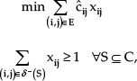
Henceforth, the above forest problem will be referred to as the primal problem, and will be used to find a lower bound and partition the targets. A dual corresponding to a linear programming relaxation (only equation (12) is relaxed to x_ij ≥0 ∀ (i, j) ∈ E) of the primal problem can be stated as follows:

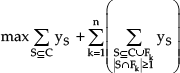
\max \sum_{S \subseteq C} y_{S} + \sum_{k = 1}^{n} (\sum_{\begin{array}{l} S \subseteq C \cup F_{k} \\ | S \cap F_{k} | \geq 1 \end{array}} y_{S})

subject to

\sum_{\begin{array}{l} S : (i, j) \in δ^{-} (S) \\ S \subseteq C \end{array}} y_{S} + \sum_{k = 1}^{n} \sum_{\begin{array}{l} S : (i, j) \in δ^{-} (S) \\ i \in C \cup F_{k} \cup {d_{k}} \\ S \subseteq C \cup F_{k}, | S \cap F_{k} | \geq 1 \end{array}} y_{S} \leq {\hat{c}}_{i j}, \forall (i, j) \in E,

(13)

y_{S} \geq 0 \forall S \subseteq C,

(14)

y_{S} \geq 0 \forall {\begin{matrix} S \subseteq C \cup F_{k}, \\ | S \cap F_{k} | \geq 1, \end{matrix} k = 1, \dots, n .

(15)

The primal-dual heuristic follows the greedy procedure outlined by Goemans and Williamson in [12]. The basic structure of this heuristic involves maintaining a forest of edges and a feasible solution to the dual problem. The edges in this forest are candidates for the set of edges that finally appear in the output of the algorithm. Initially, the forest is empty and all the dual variables are set to zero. As the forest is empty, there may be several constraints that are violated in the primal problem initially. The primal-dual heuristic is an iterative algorithm where in each iteration, the subset of vertices S corresponding to one such violated constraint in the primal problem is chosen and the dual variable y_S is increased until one of the constraints corresponding to say edge (i, j) in (13) becomes tight. A constraint corresponding to edge (i, j) becomes tight if

\sum_{\begin{array}{l} S : (i, j) \in δ^{-} (S) \\ S \subseteq C \end{array}} y_{S} + \sum_{k = 1}^{n} \sum_{\begin{array}{l} S : (i, j) \in δ^{-} (S) \\ i \in C \cup F_{k} \cup {d_{k}} \\ S \subseteq C \cup F_{k}, | S \cap F_{k} | \geq 1 \end{array}} y_{S} = {\hat{c}}_{i j} .

The algorithm then adds the edge (i, j) to the forest, and proceeds to the next iteration until the forest contains a feasible solution to the primal problem.

Once the forest becomes feasible to the primal problem, it is possible that there is more than one path from a depot to some of the targets. Therefore, in the last step of the heuristic, we eliminate some unnecessary edges in the forest while ensuring that the pruned solution is still feasible. We do this by sorting the edges in the reverse of the order in which they were added to the forest and removing them if the pruned solution is feasible to the primal problem. This pruning procedure is referred to as the reverse delete step in the literature [12], [19] and is usually used for developing good approximation algorithms for NP-Hard problems. The pseudo code of the primal-dual heuristic is presented in Algorithm 1. The key step of this primal-dual heuristic requires one to find a violated constraint (if any) in the primal problem given a forest of edges. This step is explained in the following subsection.

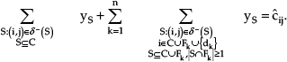
5.1 Identifying Violated Constraints

A forest is infeasible to the primal problem if there is no directed path from any of the depots to a common target or if there is no directed path from the depot d_k to any of the targets in F_k for some k ∈ {1,…,n}. If S ⊆ C and there is no incoming edge into S, then the constraint associated with S in (10) will be violated. If S ⊆C ∪ F_k, |S ∩ F_k |≥ 1 for some k∈ {1,…,n} and there is no incoming edge into S from a vertex in C ∪ F_k ∪ {d_k}, then the constraint associated with S in (11) will be violated. Henceforth, given a forest, we will refer to a set as a violated set if the forest does not satisfy the constraint associated with the set in the primal problem.

1 : All the dual variables are initially set to zero. 2 : Dual cost LB ← 0 3 : Forest T ← 4 : count ← 0 5 : while T is not feasible to the primal problem do 6 : count ← count + 1 7 : Find the set S corresponding to a violated constraint in the primal problem 8 : Increase y_S until one of the constraints corresponding to an edge e_count := (i, j) gets tight in the dual problem 9 : LB ← LB + y_S 10 : Add edge e_count to the forestT 11 : end while 12 : for k ← count down to 1 do 13 : if T\e_k is feasible then 14 : T←T\e_k 15 : end if 16 : end for 17 : Output T as a feasible solution and the dual cost (LB)as a lower bound to the primal problem

Algorithm 1. Primal-Dual Heuristic

Given a forest which is infeasible, one can use an algorithm similar to the Edmonds' algorithm [10] for the directed minimum spanning tree problem to find a violated constraint (or a violated set). Our algorithm works as follows: first, find a strongly connected component S such that S ⊆C∪F_k for some k. Contract all the arcs in this strongly connected component so that S is replaced with a single pseudo node as shown in figures 3,4. For example, in Figure 3-b, {1,7,6} is a strongly connected component and is replaced with a pseudo node in Figure 3-c. Repeat this procedure until all such strongly connected components are replaced with their corresponding pseudo nodes. Let this contracted network be denoted by G_c = (V_c, E_c) where V_c and E_c represent the set of all the vertices and edges in the contracted network respectively. Mark each vertex v in the contracted network with a label F_k if |{v}∩F_k| ≥ 1. Similarly, mark each vertex v in the contracted network with a label C if v is a common target or if v is a pseudo node such that v ⊆ C. All other vertices in V_c are unmarked. For example, in Figure 3-c, label({1,7,6})=F₁, label(2) = F₂, label(8) = C. Any graph (V',E') is a subgraph of this contracted network if V'⊆V_c and E'⊆ E_c.

Next, we repeat the following procedure for each marked vertex v in this contracted network until we find a violated set. Let G'(v) represent the largest possible subgraph of G_c such that all the vertices in G'(v) are marked, for each vertex u(≠v) in G'(v), label(u)∈ {label(v),C} and there is a directed path in G'(v) fromu to v. This subgraph can be computed using a depth first search algorithm. For example, in Figure 3-d, G'({1,7,6}) consists of just the pseudo node {1,7,6}, whereas G'(5) consists of the entire path from node 14 to node 5. Similarly, in Figure 4-d, G'({2,13}) is a forest consisting of edges (10,11), (11,{2,13}) and (12,{2,13}).

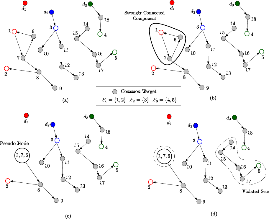
Expand each of the pseudo nodes in G'(v) and let S denote all the vertices in the expanded graph obtained from G'(v). As we ensure that the label of each of the vertices in G'(v) is either C or has the same label as v,S ⊆C∪F_k for some k. Again, referring to Figure 3, S obtained from expanding G'({1,7,6}) is equal to {1,7,6}, and S obtained from expanding G'(5) is equal to {14,15,16,17,5}.

Figure 3.

An example showing the procedure for finding the violated sets.

We output S as a violated set for the forest if label (v) = C and there is no edge directed into S. This violated set implies that its corresponding constraint in (10) is not satisfied. Similarly, we output S as a violated set for the forest if label (v) = F_k for some k and there is no edge (i,j) directed into S such that i∈C∪F_k {d_k}. This violated set implies that its corresponding constraint in (11) is not satisfied. Given a forest which is infeasible to the primal problem, one can verify that the above procedure always finds a violated cut.

6. Subgradient algorithm for addressing the Lagrangian dual problem

Given the penalty variables in λ and µ, the primal-dual heuristic presented in the previous section can be used to find a lower bound and a good, feasible solution for the Lagrangian relaxation problem in (6)–(9). In this section, we provide a subgradient algorithm for solving the Lagrangian dual problem.

The subgradient algorithm is an iterative procedure where the penalty variables are updated in each iteration based on an improving direction of the objective of the Lagrangian dual problem. Let [λ]^k and [µ]^k indicate the values of λ and µ during the k^th iteration respectively. During the k^th iteration, we compute a new set of penalty vectors, [λ]^k+1 and [µ]^k+1 using an update scheme that aims to change [λ]^k and [µ]^k along an improving direction defined by the subgradient as follows: let g_{λ_i} and g_{µ_i} denote the subgradient corresponding to the penalty variables λ_i and µ_i for i =1,…, |V| where

g_{λ_{i}} = 1 - \sum_{j \in V} x_{j i},

(16)

Figure 4.

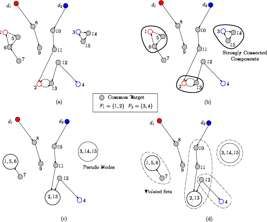
Another example showing the procedure for finding the violated sets.

g_{μ_{i}} = 1 - \sum_{j \in V} x_{i j} .

(17)

Let g = (g_λ₁,…,g_{λ_|v|},g_μ₁,…,g_{μ_|v|}) represent the vector of all the subgradients, and let [g]^k represent this vector during the k^th iteration. The new update [λ,µ]^k+1 is computed as follows:

{[λ, μ]}^{k + 1} = {[λ, μ]}^{k} + α^{k} {[g]}^{k}

(18)

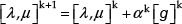
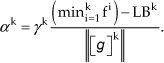
where α^k is the step size defined by

α^{k} = γ^{k} \frac{f^{*} - ϕ ({[λ]}^{k}, {[μ]}^{k})}{‖ {[g]}^{k} ‖} .

(19)

In the above equation, γ^k is a parameter in the interval (0,2], f* denotes the optimal cost of the MVP and ‖[g]^k‖ denotes the l² –norm of [g]^k. As f* may not be known, during the k^th iteration, we use the cost of the best solution found for the MVP during the first k iterations as a proxy for f*. The expression (19) is referred to as the Polyak's Rule II. A common practice is to start with a value of γ⁰ ∈(0,2] and reduce its value by a constant factor if the dual objective does not increase in a specified number of iterations [18]. The overall procedure for solving the Lagrangian dual problem is given in Algorithm 2.

1: Choose the initial penalty variables in [λ⁰, µ⁰. Let k = 0.

2: Solve the Lagrangian relaxation for [λ,µ]^k. This step would provide a lower bound LB^k to φ* (λ^k, µ^k) and a forest T^k for the primal problem.

3: Use the forest T^k to assign each target to one of the vehicles. Break the ties arbitrarily if a common target is connected to more than one depot. Once the targets have been partitioned among the vehicles, use the LKH [14] to find a corresponding path for each of the vehicles. Let the sum of the cost of travelling all the paths be denoted by f^k.

4: Terminate the algorithm if the duality gap (min^k_i=1 fⁱ - max^k_i=1 LBⁱ) is less than a constant ε, or if the number of iterations, k, has reached a maximum value; otherwise, continue to the next step.

5: Compute [λ,µ]^k+1 using equation (18), i.e., [λ,µ]^k+1 = [λ,µ]^k + α^k [g]^k. α^k is the step size given by Polyak's Rule II as follows:

α^{k} = γ^{k} \frac{({min}_{i = 1}^{k} f^{i}) - {LB}^{k}}{∥ {[g]}^{k} ∥}

In the above rule, γ⁰ is chosen to be in the interval (0,2].

For $k \geq 1, γ^{k} : = \frac{γ^{k - 1}}{2}$ if the dual objective (LB^k) does not increase in a specified number of iterations.

6: Let k ← k + 1 and go to step 2.

Algorithm 2. Subgradient algorithm for the Lagrangian dual problem

7. Computational Results

The objective of this section is to compute the quality of the solutions produced by the proposed algorithms for the MVP. In that pursuit, we conducted two sets of simulations for the MVP - in the first set, we fixed the number of vehicles and varied the number of targets; in the second set, we fixed the number of targets and varied the number of vehicles. All the simulations were run on a Dell Precision T5500 workstation (Intel Xeon E5630 processor @ 2.53 GHz, 12GB RAM).

For a given number of vehicles and targets, 50 test instances were generated. The coordinates of the targets and depots were generated randomly in a square of size 5000 m using a uniform distribution. For the simulations, we model the UV as a Dubins car that travels at a constant velocity and has a lower bound on turning radius. The minimum turning radius of all the vehicles was chosen to be equal to 250 m. For each generated target, a heading angle was selected randomly in the interval [0,2π]. The Dubins' result [9] was used to calculate the minimum distance required for a vehicle to travel between any two targets. Each vehicle was also assigned a subset containing three targets which the vehicle must visit. An upper bound on the deviation of the cost of the suboptimal solutions found by the subgradient algorithm from the optimum is defined as

100 (\frac{f^{I} - L B^{I}}{L B^{I}}),

(20)

where f^I is the cost of the best solution and LB^I is the best lower bound obtained for an instance I by the subgradient algorithm. The LKH program by Helsgaun [14] available at http://www.akira.ruc.dk/keld/research/LKH/was used to solve the HPP in the subgradient algorithm. The LKH program was run without changing any of its default settings.

While applying the subgradient algorithm to solve the Lagrangian dual problem, all the penalty variables were initially set to zero. γ⁰ was initially assigned a value of 0.001 in Equation (19), and its value was reduced by a factor of 2 whenever φ([λ]^k, [µ]^k) failed to increase in two iterations. As the iterations progresses, we can expect the best lower bound produced by the subgradient algorithm to continue to increase until it converges to a fixed value. Similarly, the cost (upper bound) of the best solution obtained by the subgradient algorithm may continue to decrease as the iterations progress. For each instance, the subgradient algorithm was allowed to run for at most 50 iterations. Figure 5 illustrates the way in which the best upper bound and the lower bound change with the number of iterations for a 30 target instance.

Figure 5.

Variation of the best upper bound and the best lower bound obtained by the subgradient algorithm as a function of the number of iterations for an instance.

In the first set of simulations, the number of vehicles was fixed to be equal to five, and the number of targets was allowed to vary from 15 to 40. The first plot in Figure 6 shows the average deviation of the cost of the suboptimal solutions produced by the algorithm from the optimum. This figure also shows the average computation time required to implement the subgradient algorithm. For the test instances considered in the first set of simulations, the proposed algorithms were able to find solutions whose cost, on an average, is at most 12% away from the optimum.

Figure 6.

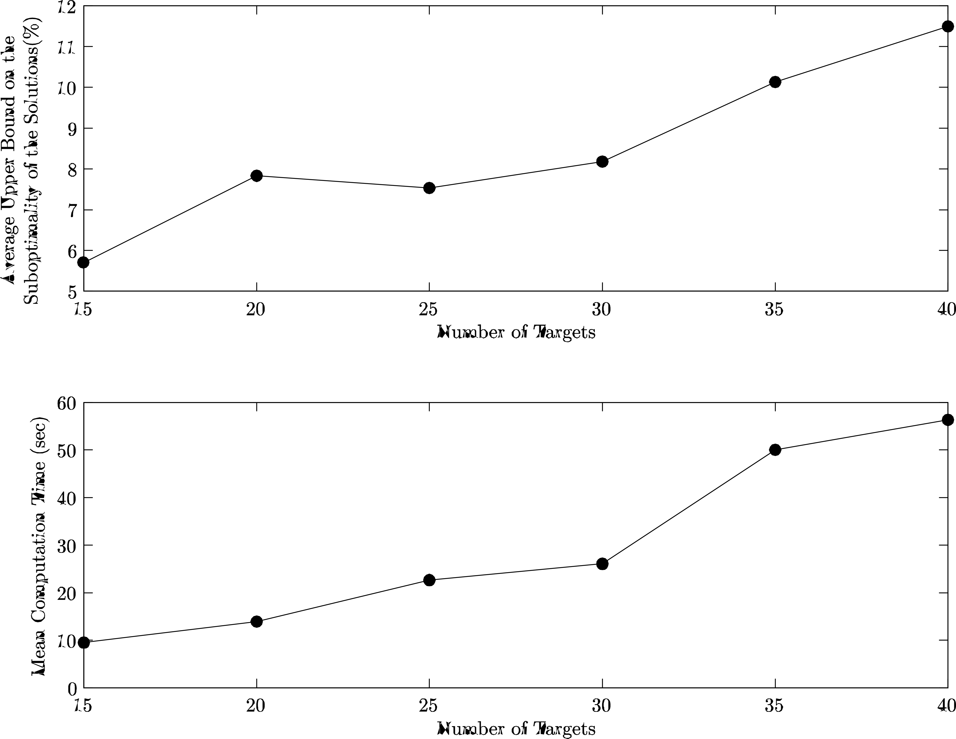
Computational results for the MVP: number of vehicles fixed.

In the second set of simulations, the number of targets was fixed at 35 and the number of vehicles was varied from 2 to 7. The first plot in Figure 7 shows the average deviation of the cost of the suboptimal solutions produced by the algorithm from the optimum. Specifically, for the test instances considered in the second set of simulations, the proposed algorithms were able to find solutions whose cost, on an average, is at most 14% away from the optimum. In addition, the average computation time required for implementing the proposed algorithms was at most equal to a minute. Considering that the MVP with additional vehicle-target constraints is a difficult problem to solve, these results indicate that the approach proposed in this article is promising. Figures 8 and 9 show the Dubins' paths found by the proposed algorithms for a couple of test instances.

Figure 7.

Computational results for the MVP: number of targets fixed.

8. Conclusion

A primal-dual heuristic was combined with the Lagrangian relaxation technique to find good solutions for a heterogeneous vehicle routing problem. Future work related to this problem can focus on two research areas. Firstly, the feasible solutions and the bounds found by the developed heuristics can be used in branch and bound solvers in order to obtain optimal solutions for the related heterogeneous vehicle routing problems. Secondly, one can aim to develop primal-dual approximation algorithms for heterogeneous travelling salesman problems where there are additional vehicle-target constraints. A result in this direction has already been reached with regard to a special case of a heterogeneous travelling salesman problem in [2].

Figure 8.

An example showing the Dubins' paths found by the algorithms for an instance with two vehicles.

Figure 9.

An example showing the Dubins' paths found by the algorithms for an instance with three vehicles.

Footnotes

10. Acknowledgements

This material is based upon work supported by the National Science Foundation under grant no. 1015066 and the Air Force Office of Scientific Research under grant no. FA9550-10-1-0392.

1

The cost of travelling for a UV from target A at an initial heading angle (ψ_A) to target B at a final heading angle (ψ_B) may be different than the cost of travelling from target B at ψ_B to target A at ψ_A.

References

The Traveling Salesman Problem and Its Variations (Combinatorial Optimization), 1 ed., Springer, May 2002.

Bae

Jungyun

Rathinam

Sivakumar

, An approximation algorithm for a heterogeneous traveling salesman problem, ASME Conference Proceedings 2011 (2011), no. 54754, 637–644.

Chandler

P.R.

Pachter

, Research issues in autonomous control of tactical UAVs, American Control Conference, 1998. Proceedings of the 1998, vol. 1, June 1998, pp. 394–398 vol.1.

Chao

I-Ming

Golden

Bruce

Wasil

Edward

, A computational study of a new heuristic for the site-dependent vehicle routing problem, INFOR (1999).

Chao

I-Ming

Liou

Tian-Shy

, A new tabu search heuristic for the Site-Dependent vehicle routing problem, The Next Wave in Computing, Optimization, and Decision Technologies ( Golden

Bruce

Raghavan

Wasil

Edward

Sharda

Ramesh

Stefan

Voß

, eds.), Operations Research/Computer Science Interfaces Series, vol. 29, Springer US, 2005, pp. 107–119.

Cordeau

Jean-François

Laporte

Gilbert

Hautes

École

, Études Commerciales, and Les Cahiers Du Gerad, A unified tabu search heuristic for vehicle routing problems with time windows, Journal of the Operational Research Society 52 (2001), 928–936.

Thomas

H. Cormen

Charles

E. Leiserson

Ronald

L. Rivest

Stein

Clifford

, Introduction to algorithms, 2 ed., The MIT Press, 2001.

Doshi

Riddhi

Yadlapalli

Sai

Rathinam

Sivakumar

Darbha

Swaroop

, Approximation algorithms and heuristics for a 2-depot, heterogeneous hamiltonian path problem, International Journal of Robust and Nonlinear Control 21 (2011), no. 12, 1434–1451.

Dubins

L. E.

, On curves of minimal length with a constraint on average curvature, and with prescribed initial and terminal positions and tangents, American Journal of Mathematics 79 (1957), no. 3, 497–516, ArticleType: Research-article / Full publication date: Jul., 1957 / Copyright © 1957 The Johns Hopkins University Press.

10.

Edmonds

, Optimum branchings, National Bureau of standards, 1968.

11.

Marshall

L. Fisher

12.

Goemans

M.X.

Williamson

D.P.

, The primal-dual method for approximation algorithms and its application to network design problems, Approximation algorithms for NP-hard problems (1997), 144–191.

13.

Held

Michael

Richard

M. Karp

, The Traveling-Salesman problem and minimum spanning trees, Operations Research 18 (1970), no. 6, 1138–1162, ArticleType: Research-article / Full publication date: Nov. Dec., 1970 / Copyright © 1970 INFORMS.

14.

Helsgaun

Keld

, An effective implementation of the Lin-Kernighan traveling salesman heuristic, European Journal of Operational Research 126 (2000), 106–130.

15.

Oberlin

Rathinam

Darbha

, Today's traveling salesman problem, Robotics Automation Magazine, IEEE 17 (2010), no. 4, 70–77.

16.

Pisinger

David

Ropke

Stefan

, A general heuristic for vehicle routing problems, Computers & Operations Research 34 (2007), no. 8, 2403–2435.

17.

Reeds

J. A.

Shepp

L. A.

, Optimal paths for a car that goes both forwards and backwards., Pacific Journal of Mathematics 145 (1990), no. 2, 367–393.

18.

Timsjo

Susanne

, An application of lagrangian relaxation to the traveling salesman problem, Tech. Rep. IMa-TOM-1999-02, Malardalen University, Department of Mathematics and Physics, Sweden (1999).

19.

David

P. Williamson

David

B. Shmoys

, The design of approximation algorithms, 1 ed., Cambridge University Press, April 2011.

20.

Yadlapalli

Bae

Jungyun

Rathinam

Darbha

, Approximation algorithms for a heterogeneous multiple depot hamiltonian path problem, American Control Conference (ACC), 2011, 29 2011-july 1 2011, pp. 2789–2794.

21.

Yadlapalli

Malik

W.A.

Darbha

Pachter

, A lagrangian-based algorithm for a multiple depot, multiple traveling salesmen problem, Nonlinear Analysis: Real World Applications 10 (2009), no. 4, 1990–1999.

A Primal-Dual Heuristic for a Heterogeneous Unmanned Vehicle Path Planning Problem

Abstract

Keywords

1. Introduction

2. Problem Statement

3. Problem Formulation

4. Lagrangian Relaxation of the MVP

5. Primal Dual Heuristic for solving the Lagrangian Relaxation

5.1 Identifying Violated Constraints

6. Subgradient algorithm for addressing the Lagrangian dual problem

7. Computational Results

8. Conclusion

Footnotes

10. Acknowledgements

1

References