View Transformation Based on a Single Outdoor Image

Abstract

Abstract An automatic approach for view transformation based on a single outdoor image is proposed in this paper. First, the hierarchical segmentation method is conducted to segment an outdoor image into several meaningful regions and each region is labelled as sky, ground or standing object. Then, different methods are used to estimate each region's depth according to its label. After that, the obtained depth information is utilized to create a new view image after any rotation, translation and pitch. Finally, the image inpainting work for the missing colour region is accomplished using its neighbour's colour. Extensive experiments show the proposed approach not only improves the accuracy of view transformation, but also performs well even for images with occlusion phenomena.

1. Introduction

Accomplishing a view transformation by utilizing a two-dimensional image is a fundamental problem in computer vision and it has important applications in 3D television, robotics, pattern recognition and other fields. A number of scholars have conducted a range of research and have achieved much.

The conventional method utilizes image-based rendering (IBR) to create new view images observed in different viewpoints [1, 2]. This method can accomplish a view transformation task in the absence of a scene geometry model, but it requires two images as input at least. Research in [3–5] achieved view transformation using the disparity between two images with slightly different projections of the same scene. These methods can complete view transformation work in real-time, but they also require two images as input at least. Research in [6, 7] proposed view transformation methods based on a colour image and its corresponding depth image. The new view images created by these methods have high accuracy, but professional equipment is necessary for obtaining the colour image and the depth image at the same time. All the aforementioned methods require two images as input at least. However, for the case where only a single two-dimensional image exists, view transformation becomes more difficult as the depth of each pixel in the image is unknown. Even so, some scholars have already put forward methods that accomplish the view transformation task based on only a single two-dimensional image.

Criminisi [8] achieved view transformation of an outdoor image by using projective geometry constrains. This method has better accuracy, but requires the user to specify a square on the ground plane, a set of “up” lines and orthogonality relationships. Horry [9] completed the view transformation task by providing a “spidery mesh” interface that required the user to label some foreground objects and to specify the vanishing point of the scene. Though this method can get better results, it still cannot accomplish the view transformation task automatically.

Recently, with the wide application of machine learning theory in image understanding, several scholars propose some automatic view transformation methods based on a single image. By using geometry features extracted from the image, Delage [10] presented a dynamic Bayesian network model for view transformation. This method can achieve satisfying results for an indoor scene with a “floor-wall” structure, but is not suitable for outdoor scenes. Saxena [11] first segmented the image into thousands of small regions. After that, the Markov random field was adopted to estimate the location and orientation of each region in different scales. Finally, the view transformation result was obtained based on the above information. This method can be applied in most outdoor scenes, but due to the inaccuracy of the estimated location and orientation, errors easily occur in the result from this method. Hoiem [12] first segmented an image into several meaningful regions and labelled each segmented region as sky, ground or standing object. These labels were then used to “cut and fold” the image into a pop-up model. Finally, the view transformation result was obtained by using this model. This method can provide a visually pleasing view transformation results for many images with simple structures, but for images with relatively complicated structures, its results are seldom satisfactory. Cao [13] proposed a close-form iteration method for image segmentation and depth estimation. This method first segmented the image into thousands of small regions. After that, region merging and depth estimation were performed alternatively in the close-form iteration process until the expected result was obtained. On this basis, each region's location and orientation were estimated by using the Markov random field. Finally, the view transformation result can be obtained by utilizing all of the above information. This method can get a slightly more visually pleasing result for an image with a relatively complicated structure, but if there is an occlusion phenomenon in the image, errors easily occur in its view transformation result.

To overcome the above deficiencies in existing methods, a novel view transformation approach is proposed in this paper. Extensive experiments show the proposed approach not only improves the accuracy of view transformation, but also performs well even for an image with an occlusion phenomenon. The rest of this paper is organized as follows. Section 2 describes the overall idea of the proposed approach and basic works. Section 3 explains the details of depth estimation and Section 4 shows the process of view transformation. Section 5 presents our experimental results and Section 6 concludes the paper.

2. Overall idea and basis works

2.1 Overall idea of proposed approach

First, colour, texture, shadow and other features extracted from the image are utilized to segment the image into several meaningful regions and each obtained region is labelled as sky, ground or standing object. Second, each region's depth is estimated according to the depth estimation method proposed later in this paper and three dimensional coordinate reconstruction of the image is performed using the depth estimation result. That is to say, for each pixel in the image, the coordinate of the real scene represented by this pixel is calculated in the world coordinate system whose origin is the initial observation position and the positive direction of the Z-axis is the initial observation direction. Third, the new observation position and direction is inputted and each point's coordinate of the real scene is calculated in the new coordinate system whose origin is the new observation position and the positive direction of the Z′-axis is the new observation direction. On this basis, each point in the new world coordinate system is projected onto the new image plane according to projective geometry theory. Lastly, the new position's colour is filled with the original pixel's colour and the image inpainting work for the missing colour pixels is completed. The specific process of the proposed approach is shown in Fig. 1.

Figure 1.

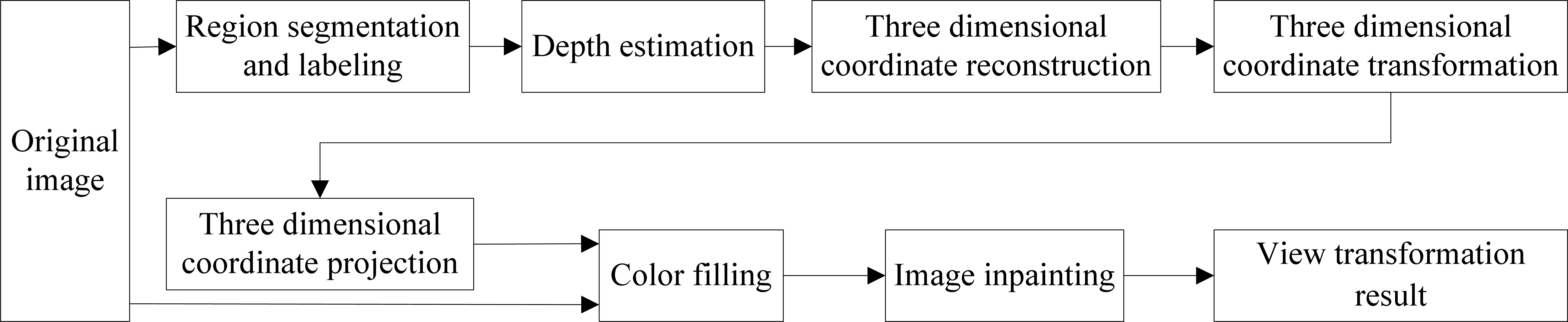
The overall process of view transformation

From Fig. 1 we can see that to get the new image after view transformation, the original image should be segmented and each segmented region's depth should be first estimated. Therefore, region segmentation and depth estimation will affect the accuracy of the view transformation directly.

2.2 Region segmentation and labelling

At present, there are several available region segmentation methods. A feature-based hierarchical segmentation method is proposed in [14]. In this method, different features are utilized in different stages to accomplish the region segmentation task and the result obtained by this method has a reasonable and good segmentation effect. Therefore, the method in [14] is adopted to segment an image into several meaningful regions in this paper. The specific region segmentation process in this paper is described as follows.

First, the watershed algorithm is adopted to segment the original image into thousands of small regions and the boundaries of all the regions are obtained. These boundaries generally contain almost all the real boundaries in the original image. Then the feature-based hierarchical segmentation method, which includes the following three operations in each iteration process, is adopted to merge the small regions.

Extract the features of regions and boundaries between regions.

Calculate all boundary strengths according to the extracted features.

Merge small regions into larger ones by removing weak boundaries whose strengths are smaller than the threshold.

Repeat the above three operations until all boundary strengths are greater than the threshold, thus the original image can be segmented into several regions, whose number is generally 3–10. On this basis, we label each region as sky, ground or standing object using a similar method to [15].

3. Depth Estimation

In general, most depth estimation methods are conducted under the assumption of no camera tilt and pitch. Under these conditions, the depth of each pixel in the image can be roughly estimated if the camera focal length and the camera height are given. Therefore, without loss of generality, the depth estimation method in this paper is also conducted under the above assumption. Let f_u and f_v represent the focal length of the camera in a horizontal and vertical orientation respectively, H_c represents the camera height, v₀ represents the ordinate of the vanishing point [16], v_p represents the ordinate of the point p to be estimated and then the depth of this point D_p can be represented as

${\mathrm{D}}_{\mathrm{p}}=\frac{{\mathrm{f}}_{\mathrm{v}}{\mathrm{H}}_{\mathrm{c}}}{{\mathrm{v}}_{\mathrm{p}}-{\mathrm{v}}_0}$

(1)

In this paper, we assume ${\mathrm{f}}_{\mathrm{u}}={\mathrm{f}}_{\mathrm{v}}=\sqrt{(im{\mathrm{h}}^2+im{\mathrm{w}}^2)/2}$ , in which imh represents the height of the image, imw represents the width of the image respectively and both of them are measured by pixels. As an image is shot by standing people generally, 1.6m is assigned to the camera height in this paper. For the region labelled as sky in the aforementioned segmentation result, its depth is assigned the farthest effective shooting distance of camera. For the region labelled as ground, the depth of each pixel is calculated by Eq. (1). For the region labelled as standing object, it is further classified into three cases of no vanishing point, vanishing point on one side or vanishing point on both sides to estimate its depth according to the vanishing point number of the region and the vanishing point location to the region. Specific methods are as follows.

(1) The case of no vanishing point

In this case, the standing object region is usually a nonplanar object, such as a plant, a person etc. Because the depth change in the region can usually be ignored, we take the depth of the lowest point in the region as the depth of the whole region.

(2) The case of vanishing point on one side

In this case, the region is usually one surface of a building and its depth usually changes gradually along the horizontal direction. Influenced by region segmentation and occlusion, the contact boundary formed by this region and the ground is not usually a straight line. Therefore, if we estimate the region depth by calculating the depth of each pixel on this boundary according to Eq. (1) directly, the estimation results will sometimes be big, sometimes small and change frequently, which does not reflect the real depth of the region. To make the estimation results more reasonable, we use the concept of a depth reference line [17]. A depth reference line is a straight line, which is fitted by the region/ground boundary and crosses the vanishing point. As shown in Fig. 2(a), the red line is the depth reference line of the yellow region with depth change. By replacing the region/ground boundary with a depth reference line to accomplish depth estimation, the phenomenon that estimation results change frequently can be avoided. Therefore, before estimating the region depth, we should determine its depth reference line first. Different from the traditional line fitting method, in this paper, Eq. (2) is utilized to determine the depth reference line, which can effectively decrease the error that arises by the detected boundary points deviating seriously from the real boundary.

Figure 2.

The sketch map of depth reference line. (a) The case of vanishing point on one side, (b) The case of vanishing point on both sides and one sub-region is occluded and (c) The case of vanishing point on both sides and neither of the two sub-regions is occluded.

$\underset{\mathrm{k},\mathrm{b}}{\min }\hspace{1em}{\displaystyle \sum _{\mathrm{i}=1}^{\mathrm{n}}\log (\frac{\left|\mathrm{k}{\mathrm{u}}_{\mathrm{i}}-{\mathrm{v}}_{\mathrm{i}}+\mathrm{b}\right|}{\sqrt{1+{\mathrm{k}}^2}}}+1)\hspace{1em}\mathrm{s}.\mathrm{t}.\hspace{0.17em}\hspace{1em}\mathrm{k}{\mathrm{u}}_0-{\mathrm{v}}_0+\mathrm{b}=0$

(2)

Where k is the slope of the depth reference line, b is the intercept of the depth reference line on the ordinate axis of the image coordinate system, n is the pixel number on the region/ground boundary, (u_i, v_i) is the coordinate of the ith pixel on the boundary and (u₀, v₀) is the coordinate of the vanishing point corresponding to this region. After obtaining the depth reference line, the depth of each pixel on the depth reference line is calculated by Eq. (1). Finally, according to the rule that the depth of pixel along the vertical direction of the image is equal, the depths of all pixels in the region are determined based on the depths of pixels on the depth reference line.

(3) The case of vanishing point on both sides

In this case, the region is usually two intersecting surfaces of a building and each surface's depth changes gradually along the horizontal direction. To estimate this region's depth, the ridge formed by the two surfaces of the building is found by using Hough transform and image texture gradient firstly, as shown in Fig. 2(b) and Fig. 2(c). In Fig. 2(b) and Fig. 2(c), the ridge divides the standing object region into two sub-regions A and B and each sub-region's depth increases or decreases along the horizontal direction. After that, the depth reference line of each sub-region is determined respectively. While determining the depth reference lines, we need to judge whether there is a visible sub-region/ground boundary in both sub-regions. If there is a visible sub-region/ground boundary in only one sub-region, it shows another sub-region has been occluded by other region(s), as shown in Fig. 2(b), where the sub-region A has been occluded by the green region. In this case, we should determine the depth reference line of the sub-region with a visible sub-region/ground boundary first, as the red solid line shown in Fig. 2(b), then determine the intersecting location of the ridge and ground using this depth reference line and take the line connecting the intersecting location and the other vanishing point as the depth reference line of the sub-region without a visible sub-region/ground boundary, as the red dashed line shows in Fig. 2(b). If there are visible sub-region/ground boundaries in both sub-regions, the depth reference line of each sub-region is determined and its fitting degree with the boundary is calculated respectively. In this case, as the intersections of the ridge and two depth reference lines may not coincide, to avoid the depth ambiguity of the ridge, we need to adjust one of the depth reference lines. In this paper, we take the intersection of the ridge and the depth reference line with a higher fitting degree as the final intersection and the line connecting this final intersection and the other vanishing point is taken as the depth reference line of the other sub-region, as shown in Fig. 2(c). In Fig. 2(c), the ridge divides the standing object region into two sub-regions A and B. The green and the red solid lines are the depth reference lines of A and B, calculated by Eq. (2), respectively. Due to fact that the depth reference line of region B has a higher fitting degree, the intersection of this depth reference and the ridge is taken as the final intersection of the ridge and ground and the line connecting the final intersection and the other vanishing point is taken as the final depth reference line of sub-region A, as the red dashed line shows in Fig. 2(c). Then, the depth of each pixel on both depth reference lines is calculated by Eq. (1). Finally, according to rule that the depth of a pixel along the vertical direction of the image is equal, the pixel depth in each region is determined based on its depth reference line respectively.

4. View Transformation

After each pixel's depth has been estimated, it can be used to conduct a view transformation, as shown in Fig. 3.

Figure 3.

The sketch map of view transformation

In Fig. 3, o represents the initial observation position, c represents the image plane centre of the initial observation position, o'represents the new observation position, c′ represents the image plane centre of the new observation position, p(u,v) is a pixel in the original image and P(x,y,z) represents the actual position of pixel p(u,v) in the real scene. The goal of view transformation is to determine the new position p′(u′,v′) of pixel p(u,v) in the new view image and fill it with the colour information of pixel p(u,v), at the same time, performing image inpainting for the missing colour region. To achieve the above goal, four steps are conducted in this paper. First, three dimensional coordinate reconstruction is performed by using the obtained depth estimation result. That is to say, for each pixel p(u,v), calculate the coordinate P(x,y,z) of the real scene represented by this pixel in the world coordinate system O-XYZ whose origin is the initial observation position and the positive direction of the Z-axis is the initial observation direction. After that, input the new observation position and direction and calculate the new coordinateP(x′,y′,z′) of P(x,y,z) in the new world coordinate system O′-X′Y′Z′ whose origin is the new observation position and the positive direction of the Z′-axis is the new observation direction. On this basis, calculate the position p′(u′,v′) of the point P(x′,y′,z′) in the new image plane. Lastly, fill the colour of the new position p′(u′,v′) with the colour of the pixel p(u,v) and complete the image inpainting work for the missing colour region. The specific procedure is described as follows.

4.1 Three dimensional coordinate reconstruction

Let D represent the depth of pixel point p. Then according to projective geometry principles we can calculate the point P(x,y,z)'s coordinate in the world coordinate system using the pixel p(u,v)'s coordinate in the image coordinate system, as shown in Eq. (3).

$\left(\begin{array}{c}\mathrm{x}\\ \mathrm{y}\\ \mathrm{z}\end{array}\right)=\left(\begin{array}{ccc}{\mathrm{d}}_{\mathrm{x}}& 0& 0\\ 0& -{\mathrm{d}}_{\mathrm{y}}& 0\\ 0& 0& {\mathrm{D}}_{\mathrm{p}}\end{array}\right)\left(\begin{array}{c}\mathrm{u}\\ \mathrm{v}\\ 1\end{array}\right)$

(3)

In Eq. (3), u and v represent the abscissa and ordinate of pixel point pin the image coordinate system respectively. d_x represents the horizontal distance of each pixel in the world coordinate system, which can be calculated by d_x = D_p / f_u . d_y represents the vertical distance of each pixel in the world coordinate system, which can be calculated by d_y = D_p / f_v.

4.2 Three dimensional coordinate transformation

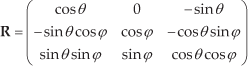
On the basis of each pixel's coordinate in the world coordinate system calculated above, the coordinate of each pixel in the new world coordinate system can be obtained according to the new observation position and observation direction. Let the new observation position be the origin and the new observation direction be the positive direction of the Z′-axis of the new world coordinate system. Then each point P(x,y,z)'s coordinate P(x′,y′,z′) in the new world coordinate system can be represented by the rotation angle θ from the initial observation direction to the new observation direction around the Y-axis, the pitch angle ϕ around the X axis and the translation vector t from the initial observation position to the new observation position (the tilt angle ϕ from the initial observation direction to the new observation direction around the Z-axis can always be ignored because it is of no practical significance).

Let R be the rotation matrix from the world coordinate system O-XYZ to O′-X′Y′Z′. Then the rotation matrix R can be represented by rotation angle θ and pitch angle ϕ, as shown in Eq. (4).

$\mathbf{R}=\left(\begin{array}{ccc}\cos \theta & 0& -\sin \theta \\ -\sin \theta \cos \phi & \cos \phi & -\cos \theta \sin \phi \\ \sin \theta \sin \phi & \sin \phi & \cos \theta \cos \phi \end{array}\right)$

(4)

Let t = (t_x,t_y,t_z)^T represent the translation vector for the initial observation position to the new observation position. Then the new coordinate P(x′,y′,z′) of point P(x,y,z) in the new world coordinate system O′-X′Y′Z′ can be represented by Eq. (5).

$\left(\begin{array}{c}\mathrm{x}\text{'}\\ \mathrm{y}\text{'}\\ \mathrm{z}\text{'}\\ 1\end{array}\right)=\left(\begin{array}{cc}\mathbf{R}& \mathbf{t}\\ 0^{\mathrm{T}}& 1\end{array}\right)\left(\begin{array}{c}\mathrm{x}\\ \mathrm{y}\\ \mathrm{z}\\ 1\end{array}\right)$

(5)

Eq. (5) can also be represented as Eq. (6) if we substitute the rotation matrix R and the translation vector t into it.

$\left(\begin{array}{c}\mathrm{x}\text{'}\\ \mathrm{y}\text{'}\\ \mathrm{z}\text{'}\\ 1\end{array}\right)=\left(\begin{array}{cccc}\cos \theta & 0& -\sin \theta & {\mathrm{t}}_{\mathrm{x}}\\ -\sin \theta \cos \phi & \cos \phi & -\cos \theta \sin \phi & {\mathrm{t}}_{\mathrm{y}}\\ \sin \theta \sin \phi & \sin \phi & \cos \theta \cos \phi & {\mathrm{t}}_{\mathrm{z}}\\ 0& 0& 0& 1\end{array}\right)\left(\begin{array}{c}\mathrm{x}\\ \mathrm{y}\\ \mathrm{z}\\ 1\end{array}\right)$

(6)

4.3 Three dimensional coordinate projection and colour filling

On the basis that each pixel's coordinate in the new world coordinate system O′-X′Y′Z′ has been calculated, each pixel's position in the new view image can be determined according to projective geometry principles, as shown in Eq. (7).

$\left(\begin{array}{c}\mathrm{u}\text{'}\\ \mathrm{v}\text{'}\\ 1\end{array}\right)=\left(\begin{array}{ccc}\frac{1}{{\partial }_{\mathrm{x}}}& 0& 0\\ 0& -\frac{1}{{\partial }_{\mathrm{y}}}& 0\\ 0& 0& \frac{1}{\mathrm{z}\text{'}}\end{array}\right)\left(\begin{array}{c}\mathrm{x}\text{'}\\ \mathrm{y}\text{'}\\ \mathrm{z}\text{'}\end{array}\right)$

(7)

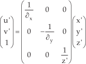
In Eq. (7), u′ and v′ represent the abscissa and ordinate of pixel point p in the new image coordinate system respectively. (x′,y′,z′) represents the point P(x,y,z)'s coordinate in the new world coordinate system O′X′Y′Z′. ∂_x represents the horizontal distance of each pixel in the world coordinate system, which can be calculated by ∂_x = z′/f_u. ∂_y represents the vertical distance of each pixel in the world coordinate system, which can be calculated by ∂_y = z′/f_v.

Once each pixel's position in the new view image has been determined, the new position can be filled with the colour of its corresponding pixel in original image. In this process, due to the existence of occlusion phenomena in the original image, several pixels may have the same projection position in the new view image. In this case, we fill the new position with the colour of the pixel with a smaller depth, because the pixel with a smaller depth generally occludes the pixel with a bigger depth.

4.4 Image inpainting for the missing colour region

Due to the fact that the coordinate of each pixel in the new image coordinate system must be integer, the rounding operation is necessary for the coordinate of p′(u′,v′) in Eq. (7), thus some pixels' colour will be missing after colour filling as is shown by the black lines in Fig. 4(e). In addition, the existence of occlusion phenomena in the image may also make the occluded region visible in the new view image. In this condition, some regions' colour will also be missing due to the absence of the colour information of the occluded region, as the continual black region highlighted by the red rectangle shows in Fig. 4(e). Therefore, to obtain a satisfactory result, we need to perform image inpainting for the missing colour regions.

Figure 4.

View transformation results in different stages of the proposed approach

For the missing colour regions caused by the rounding operation, the colour can be repaired by a mean filter using the colour information of its 8-neighborhood pixels. For the missing colour region caused by occlusion phenomena, the repairing process is described as follows.

To avoid the missing colour region being filled with foreground region's colour (the standing object region that is adjacent to the missing colour region and has the smallest depth is regarded as the foreground region, the others are regarded as background regions in this paper), we perform a morphological dilation operation on the missing colour region to expand the area of the region. The cross type kernel function is chosen in this paper.

For each pixel in the missing colour region after dilation, its colour is repaired with the colour information of its 24-neighborhood pixels. As the camera tilt can always be ignored in the process of view transformation and the missing colour region's colour has higher similarity with its neighbouring pixels in the horizontal direction, higher weights are assigned to the pixels adjacent to the missing colour region on horizontal direction when we perform image impainting. For example, when we perform image inpainting for pixel p, its 24-neighborhood pixels' weights are shown in Eq. (8).

$\mathrm{W}=\frac{1}{36}\left(\begin{array}{ccccc}0& 1& 2& 1& 0\\ 1& 2& 3& 2& 1\\ 3& 4& \mathrm{p}& 4& 3\\ 1& 2& 3& 2& 1\\ 0& 1& 2& 1& 0\end{array}\right)$

(8)

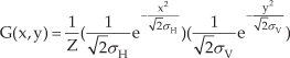
To make the new view image reflect the real scene more accurately, we apply an asymmetric Gaussian smoothing function in Eq. (9) to the missing colour region. Experimental results show that the new view image has the best effect with the horizontal standard deviation σ_H = 40 and the vertical standard deviation σ_V = 20.

$\mathrm{G}(\mathrm{x},\mathrm{y})=\frac{1}{\mathrm{Z}}(\frac{1}{\sqrt{2}{\sigma }_{\mathrm{H}}}{\mathrm{e}}^{-\frac{{\mathrm{x}}^2}{\sqrt{2}{\sigma }_{\mathrm{H}}}})(\frac{1}{\sqrt{2}{\sigma }_{\mathrm{V}}}{\mathrm{e}}^{-\frac{{\mathrm{y}}^2}{\sqrt{2}{\sigma }_{\mathrm{V}}}})$

(9)

4.5 View transformation algorithm

The proposed view transformation algorithm is described as follows.

Input: Original image

Output: View transformation result

Step1: Segment the original image into several regions by hierarchical segmentation method

Step2: Label each segmented region as sky, ground or standing object

Step3: For each segmented region k = 1 to n {

If Label(k) = sky | ground

Estimate its depth by the sky or ground region's depth estimation method

Else {

If VanishingPoint(k) = 0

Take the lowest point's depth as the whole region's depth

Else VanishingPoint(k) = 1 | 2

Estimate the region's depth by its depth reference line

}

}

Step4: For each pixel of the original image p = 1 to total {

Calculate its new position p′ on new image plane according to the obtained depth information

// Fill colour in the new image plane point-by-point by row

// One p′ maybe have several corresponding p due to the existence of occlusion phenomenon

If (Colour(p′) = null) | (Depth(p′) < Depth(p_previous))

// If the new position's colour has not been filled or the depth of p′ is smaller than the depth of the previous pixel that is utilized to fill the new position

Fill p′ with the colour of p in the original image

}

Step5: For each pixel in the new image p′ = 1 to total {

// Handle missing colour pixels caused by rounding operation or occlusion phenomenon

If Colour(p′) = null

Repair its colour with the image inpainting method proposed in Section 4.4

}

5. Experiment and analysis

5.1 Experiment scheme

We searched “Campus”, “City”, “Outdoor” and “Street” on Google and downloaded 150 images as experiment dataset. Running on a computer with 32-bit Intel core i5 2.67GHz, 1.79 GB available memory and Matlab 2010(a) environment, our approach took about 280 seconds for an 800×600 image, of which 170 seconds was for region segmentation, 10 seconds was for region labelling, 80 seconds was for depth estimation, 15 seconds was for view transformation and 5 seconds was for image inpainting. Taking an image with occlusion phenomenon as an example, the results in different stages of the proposed approach are shown in Fig. 4.

5.2 Comparison and analysis

To evaluate the performance of the proposed view transformation approach, we conduct contrastive experiments with Saxena [11], Hoiem [12] and Cao [13]. Comparison experiments are carried out in two aspects.

• (A)

To validate whether the proposed view transformation approach performs better for images with planar standing object regions, the dataset is divided into two subsets (with and without planar standing object regions) and both of them are tested by the above four methods respectively. In our experiment dataset, there are 34 images without planar standing object regions. Saxena [11], Hoiem [12], Cao [13] and the proposed approach perform best on 8, 6, 11 and 9 images, which take 23.53%, 17.65%, 32.35% and 26.47% of all the above 34 images in our dataset, respectively, as the blue histogram shows in Fig. 5. In Fig. 5, the ordinate axis indicates the percentage of the corresponding method's view transformation results, which perform best in all the four methods for each kind of region. For all of the remaining 116 images with planar standing object regions, Saxena [11], Hoiem [12], Cao [13] and the proposed approach perform best on 13, 16, 26 and 61 images, which take 11.21%, 13.79%, 22.41% and 52.59% of all the rest 116 images, respectively, as the light blue histogram shows in Fig. 5.

(B)

To validate the performance of different methods for occlusion phenomena, we divide the dataset into two subsets called with and without occlusion phenomena, which have 92 and 58 images respectively. On this basis, we use the same method as described in (A) to calculate the performance of the four different view transformation methods. Experimental results show that for the 58 images without occlusion phenomena, Saxena [11], Hoiem [12], Cao [13] and the proposed approach perform best on 14, 13, 16 and 15 images, which take 24.14%, 22.41%, 27.59% and 25.86% of all the above 58 images in our dataset, respectively. However, for the other 92 images with occlusion phenomena, Saxena [11], Hoiem [12], Cao [13] and the proposed approach perform best on 8, 17, 11 and 56 images, which take 8.69%, 18.48%, 11.96% and 60.87% of all the above 92 images in our dataset, respectively. The comparison result is shown in Fig. 5 with yellow and brown histograms respectively.

Figure 5.

Comparison result of different view transformation methods

From the above analysis we can conclude that for the images without planar standing object regions and the images without occlusion phenomena, the proposed approach performs almost the same as other methods. But for the images with planar standing object regions, our depth estimation results are more accurate due to each standing object's depth being estimated according to its vanishing point number and the vanishing point's location to the region. Thus our view transformation results based on this depth estimation results are more close to reality than other methods. Specific experiment results are shown in Fig. 6. Also, because we take occlusion into consideration in the process of view transformation, our view transformation approach can obtain more accurate results for the images with occlusion phenomena. The experiment results are shown in Fig. 7.

Figure 6.

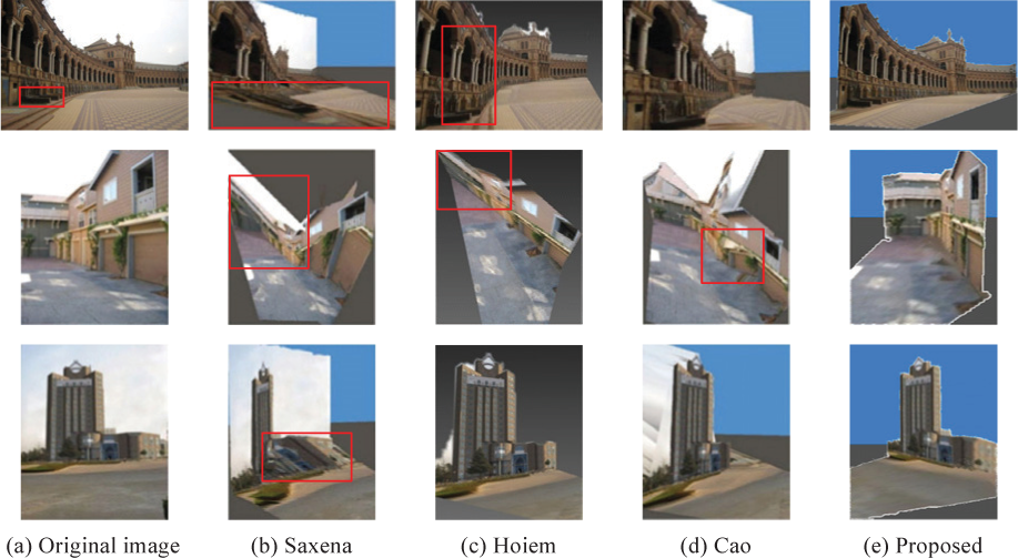
Results of different view transformation methods for images with planar standing object regions

Figure 7.

View transformation results of images with occlusion

In Fig. 6, column (a) shows the original images, column (b) shows the results of Saxena's method [11], column (c) shows the results of Hoiem's method [12], column (d) shows the results of Cao's method [13] and column (e) shows the results of the proposed method. Due to the inaccuracy of Saxena's method [11] in estimating each of the small region's locations and orientations by using a Markov random field, some regions will be stretched in the new view image, as the red boxes show in column (b). Hoiem [12] estimates each standing object's depth by applying Eq. (1) on the region/ground boundary directly, therefore errors easily occur in its depth estimation result when there is a protuberance on the region/ground boundary, as the red box shows in column (a). It will further affect the accuracy of the view transformation result, as the red box shows in the first row of Fig. 6(c). In addition, because of not taking the intersection of two planar standing object regions into consideration both in depth estimation and the view transformation process, Hoiem's method [12] incorrectly regards the two intersecting planar standing object regions as one planar standing object region, as the red box shows in the second row of Fig. 6(c). By completing the region merging and depth estimation work in a close-form way, Cao [13] effectively reduces the error generated in the process of estimating each small region's location, thus the phenomenon that some regions will be stretched in the new view image is avoided. However, because this method still generates a relatively higher error rate in estimating region orientation, Cao [13] incorrectly considers some regions on the same standing object plane to have different orientations, as the red box shows in the second row of Fig. 6(d). By taking different methods to finish the standing object region's depth estimation work according to vanishing point information, the proposed approach can obtain a more accurate depth estimation result. On this basis, each pixel's position in the new view image can be uniquely determined by the proposed view transformation approach, thus the new view image will be more accurate, as the results shown in column (e).

Among all the three methods proposed by Saxena [11], Hoiem [12] and Cao [13], Hoiem's method [12] has the best effect for the images with occlusion phenomena. Therefore, to verify the validity of the proposed approach in tackling the image with occlusion phenomena, we perform a contrastive experiment between our approach and Hoiem's method [12]. Due to accomplishing region segmentation only through a single iteration, Hoiem's method [12] cannot segment the pedestrians and the ground into different regions, so the pedestrians' depth can only be estimated using the depth estimation method for the ground region. Therefore, the occlusion phenomenon between the pedestrians and the ground cannot be detected, which will further lead to errors in the view transformation result. In Fig. 7(a), there are apparent occlusion phenomena between the pedestrians and the ground, but Hoiem [12] incorrectly considers the pedestrians to be in the ground rather than on it, as shown in Fig. 7(b). By utilizing a hierarchical segmentation method to segment the image into several meaningful regions through three iterations, the proposed approach can effectively segment the pedestrians, the ground and the standing object into different regions, as shown in Fig. 4(b). Therefore, the pedestrians' depth can be estimated using the depth estimation method for the standing object region and the occlusion relationship between the pedestrians and the ground can be determined according to the principle that the region with smaller depth occludes the other. Furthermore, as we take occlusion phenomena into consideration in the process of view transformation and use its neighbour's colour to complete the image inpainting work for the missing colour region, our results reflect the real scene more correctly. Therefore, the proposed approach can correctly determine the pedestrians' location in the new view image, as shown in Fig. 7(c).

6. Conclusions

In this paper, we propose a novel view transformation approach using only a single outdoor image and describe it in detail. The work is distinguished by two contributions. (1) An automatic view transformation method for creating the new view image after any rotation, translation and pitch is presented, which overcomes the deficiencies in existing methods that cannot handle occlusion effectively. (2) An image inpainting method for missing colour regions of the new view image are proposed, which can handle the missing colour region caused by both the rounding operation and occlusion phenomena effectively. Extensive experiment results show that, compared with other methods, the proposed approach not only can accomplish the view transformation task automatically, but also performs well for the images with apparent occlusion.

7. Acknowledgments

We would like to thank the anonymous reviewers for their helpful suggestions. This work is supported by the State Key Laboratory of Robotics and Systems (HIT), under Grant No. SKLRS-2010-ZD-08, the National Natural Science Foundation of China, under Grant No. 60975062 and the Natural Science Foundation of Hebei province, under Grant No. F2010001276.