Learning Representative Features for Robot Topological Localization

Abstract

This paper proposes a new method for mobile robots to recognize places with the use of a single camera and natural landmarks. In the learning stage, the robot is manually guided along a path. Video sequences are captured with a front-facing camera. To reduce the perceptual alias of visual features, which are easily confused, we propose a modified visual feature descriptor which combines the dominant hue colour information with the local texture. A Location Features Vocabulary Model (LVFM) is established for each individual location using an unsupervised learning algorithm. During the course of travelling, the robot employs each detected interest point to vote for the most likely place. The spatial relationships between the locations, modelled by the Hidden Markov Model (HMM), are exploited to increase the robustness of location recognition in cases of dynamic change or visual similarity. The proposed descriptors are compared with several state-of-the-art descriptors including SIFT, colour SIFT, GLOH and SURF. Experiments show that both the LVFM based on the dominant Hue-SIFT feature and the spatial relationships between the locations contribute considerably to the high recognition rate.

1. Introduction

Global localization in the operation environment is a fundamental and challenging capability for any robot exhibiting goal-oriented behaviour. The basic methodology for self-localization is to compare sensor information with previously captured knowledge about the environments. The self-localization problem [1, 2, 3, 22, 23] has been studied carefully in the field of mobile robotics and a variety of approaches with different sensors and capabilities have been developed. Research into robot localization has diverged into different schemes, which are either based on geometric models [4, 5], a topological map [6, 7] or some hybrid method.

The geometric approaches that utilize metric maps allow the robot to keep track of its exact position with respect to the map's coordinate system. Most geometric approaches rely on an Extended Kalman Filter (EKF) that needs good statistical models of the sensors and their uncertainties. In some cases, situations where the robot travels over a bump (e.g. a cable lying on the floor) are difficult to model [4]. This scheme is vulnerable to inaccuracies and expensive computation, especially in large-scale environments.

While topological approaches can be considered as an abstraction of the real world in the form of a graph, the robot's location is given by a node without metric information, i.e., there is no need to measure the coordinates of the environments. So the memory size can be reduced and it can be used in large-scale environments. The topological approaches guarantee robust performance against getting lost due to the multi-modal representation of the robot's position [6].

The extrinsic sensors are required to provide rich information to reliably distinguish between adjacent locations, for a robust localization system. Most of the early work on place recognition was based on sonar. Recent advances in robot vision have made the fusion of vision and other range sensors a viable modality, opening up possibilities for more robust detection. The task of vision-based topological localization for mobile robots is to automatically associate images with semantic labels. We expect that monocular vision itself can provide sufficient information without the need of additional sensors such as stereo sensors [4], sonars [5] or a laser rangefinder.

The landmark based methods are preferred for their simplicity. In such methods, the descriptions of the robot's surroundings could make better use of the topology of the environment, using less memory [7, 8, 9]. However, covering the environment with artificial landmarks requires modifying the environments. Corners, doors, overhead lights, markers installed on the surface of the tanker or air diffusers in ceilings [6] are used as natural landmarks. Zhu et al. [22] integrated visual landmark matching to a pre-built landmark database in a visual-inertial navigation system with front and back facing calibrated stereo cameras. In [23], Andreas Wendel designed a MAV monocular localization system based on natural landmarks, which allows global registration directly. Most of the robotic systems which use landmarks are tailored for specific situations. They can rarely be easily generalized for use in different environments.

Natural landmarks are usually detected by the technique of interest points and characterized by local feature descriptors. Local image features have received a lot of attention in recent years and they have already gained popularity and dominance in object recognition tasks nowadays. Local features could be more discriminative and robust to image variations and clutter, scene dynamics and partial occlusion compared to global ones. There are a number of state-of-the-art descriptors, including Scale Invariant Feature Transform (SIFT) [10, 11, 25], colour SIFT [20], Centre-Symmetric Local Binary Pattern (CS-LBP) [24], Histogram of Oriented Gradient (HOG) [21], Speeded-Up Robust Features (SURF) [19], Gradient Location and Orientation Histogram (GLOH) [11]. GLOH, SURF, HOG, colour SIFT can be seen as various extensions or refinements of SIFT. These descriptors are dominant because they are able to capture local visual content characterizations through the distribution of intensity gradients. As is well known, the downside of SIFT and colour SIFT, especially the colour SIFT, is the high computational cost.

In this paper, a simplified colour SIFT descriptor is designed and adopted to recognize natural landmarks for its effective invariant attribute. We should take advantage of the invariant attribute and keep the number of reference features in the database to a minimum to reduce memory. Another desirable property of this natural landmark feature is that it can easily be trained in different environments.

This paper is organized as set out below. The next section describes the problem of the existing method and the outlines of the proposed method. Details of the environment modelling are presented in section 3, which involves modified local invariant features, dimension reduction, the Roust Rival Penalized Competitive Learning (RPCL) clustering algorithm and the construction of a “Location Features Vocabulary Model” (LFVM) for each location. How the LFVMs are used to localize a robot in a topological graph using the voting method and HMM is described in section 4. Section 5 gives details about the results of the comparative experiments. The proposed descriptors are compared with several state-of-the-art descriptors including SIFT, colour SIFT, GLOH and SURF. Conclusions and discussions are given in the last Section, 7.

2. Outlines of Our Approach

Topological localization refers to the identification of the discrete location of the robot. Traditionally, most systems [6, 12]associate the reference images with the corresponding locations in the training stage. They are concerned with matching the captured image against the set of model images according to similarities between the detected features and those in the reference images. The robot moves autonomously along the path while localizing itself by performing a comparison between the learned and acquired views. The place, the model image of which best matches the input view, is then considered to be the right position. In this approach, vision based topological localization is treated as an image retrieval task [6]. The aim of the method is to determine the model view that is most similar in appearance to the current captured view.

How the known approaches will perform in the new environments is a debated and open problem. The proposed approach is different from other existing ones. In our approach, it is not necessary to match new images with one or more pre-recorded reference images, but will be matched with the feature-set pooled within the corresponding place. Our approach is motivated by an analogy with learning methods using the bag-of-words [13] representation for text categorization and probabilistic localization [14]. The idea of adapting text categorization methods to visual categorization is not new. For example, an object class recognition method is proposed [12] for the unsupervised learning of invariant descriptors of image windows. However, in the training step of their method, distinct views of the same object class must be segregated into different categories. In our approach, test images, the view angles of which are significantly different from the training views, can be classified into the same class that they would be if these images belonged to the same location.

Probabilistic algorithms [14, 15] deal with uncertainties and sensor errors, hence they allow the robot to recover from the kidnapped problem, and have been widely applied in the global localization problem. The authors make use of the probabilistic integration of the appearance and odometry data [2] to cope with the absence of reliable sensor information.

As many researchers have done previously, the the interesting points of the discriminative SIFT are selected as visual natural landmarks in the training images. However, there are a lot of similar or identical interest points in these consecutive training images. The volume of the high dimensional landmarks database is enormous and this may consequently produce many problems such as redundant feature matching and a heavy burden in searching for the right landmarks. Hence, a redundant reduction strategy in the dataset is necessary in order to build a more compact feature space.

The outline of the proposed algorithm is illustrated, separated into an off-line training stage and an on-line testing stage respectively, in the bottom and top part of Fig. 1. The physical layout of the large office environment is shown in Fig. 2. Firstly, the robot is manually guided along a route during a training step. The image sequence captured by the robot camera is divided into individual locations. At the environment modelling stage, the focus of our approach is how to build a compact and, at the same time, discriminant feature-set model that is suitable for representing each individual location. Such feature-set models consist of discriminative local features from different images that are captured from various viewpoints, scales and lighting conditions.

Figure 1.

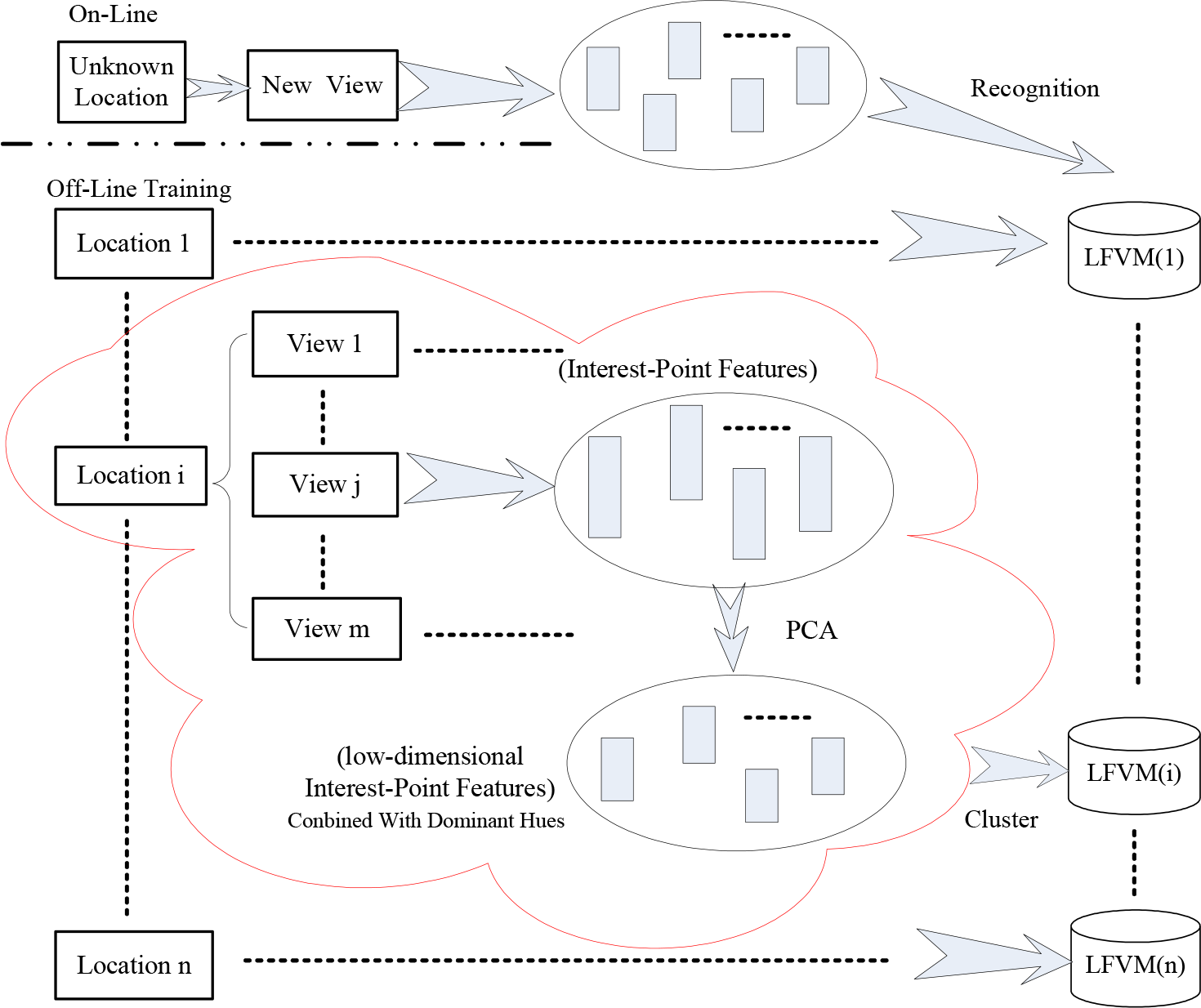
Framework of the proposed method. For each individual location, a LFVM is learned from all the available key-points detected in multiple reference images associated with the same place

Figure 2.

Physical layout of the test environment which is segmented into 19 labelled places

Figure 3.

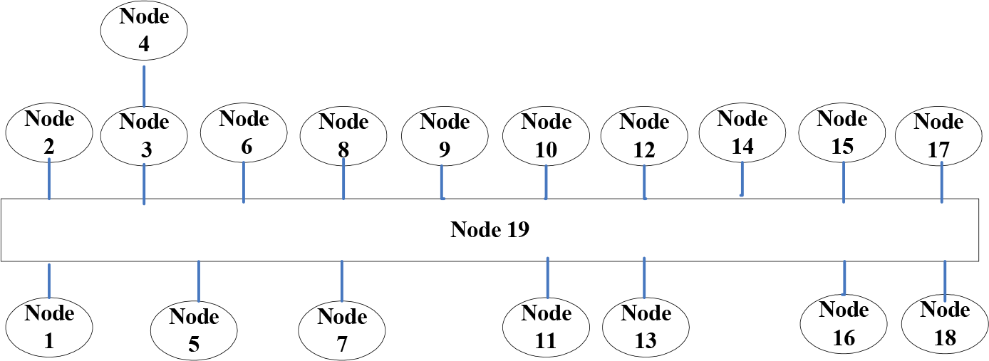
Topological graph as an abstract representation of the environment shown in Figure 2, and labels associated with the individual locations

Figure 4.

In the training step, some views of the reference images are listed, that belong to exactly the same place: the elevator lobby, which is modelled as the node “lift2” in the topological graph, as shown in Fig.2

The following procedures are conducted to perform robot self-localization in the topological map:

1. The key-points in the training images are extracted and described;

2. The feature space is compressed in two directions by utilizing Principal Component Analysis (PCA) and a Robust Rival Penalized Competitive Learning (RPCL) algorithm. Such a compact low-dimensional feature space constructs the “Location Features Vocabulary Model” (LFVM) for each individual topological node (place);

3. The key-points in the current acquired image are detected from the camera video and the index of the location is determined (the right class);

4. The neighbourhood relationship between individual locations is modelled by a Hidden Markov Model (HMM), which can be used to improve the location recognition rate.

3. Environment Modelling

As the first step of our method, the environment model is built in the exploration stage. The space is defined as a topological graph where all the nodes and arcs correspond to a group of locations and neighbourhood relationships or linkages between them. Each location is associated with a corresponding “Location Features Vocabulary Model” (LFVM) by learning the modified visual features. The method for building such a model is illustrated in Fig. 1.

The application of vision sensors in robotics always raises the problem as to which kind of image features would be most discriminative. Though some researchers have applied omni-directional cameras as their vision sensors, a regular camera is utilized in this paper. It is often argued that local feature-based representations are more robust against scene dynamics, background clutter and partial occlusion than globally derived features. A popular approach for obtaining local visual features that have robust attributes is known as “interest point” detection, which involves identifying interest points that can be reliably extracted from various viewpoints of the same scene. In this paper, we propose a modified feature descriptor, that combines the SIFT feature with dominant hue information, as a special natural landmark in single camera vision.

3.1. Composite Visual Feature

SIFT is proposed in [10] as a smart technique for detecting and describing key-points which are invariant to ordinary image transformations. Standard SIFT descriptors take 16 orientation histograms aligned in a 4×4 grid. Each histogram in each grid has 8 orientation bins where each is created over a support window of 4×4 pixels. The resulting feature vector is composed of 128 elements with a total support window of 16×16 scaled pixels. The simplified SIFT version with 2×2 grids is depicted in [10]. Owing to its effective invariant properties, SIFT has been successfully used in various tasks, including object recognition/categorization, content based image retrieval and other computer vision applications. Mikolajczyk and Schmid [11] have shown that, of several current widely used interest point descriptors, SIFT is the most effective in retaining consistency across wide variations in viewpoint and scale.

However, the SIFT feature is designed mainly for gray images and ignores important colour content. Colour information can provide valuable information in object detection and recognition tasks. Lots of objects can be misclassified if their colour cues are omitted. Some authors make use of the standard SIFT algorithm in each colour channel of the RGB colour space respectively; they then combine the individual results in a weighted manner. The primary drawback of this method is a relatively high computational burden that is three times that of the typical SIFT.

The standard SIFT features detected in two consecutive views belonging to the same location (but with different view angles) are shown in Fig. 5 (a) and (b). It demonstrates that the standard SIFT features are insensitive to changes in viewpoint. We can see from Fig. 6 that, although most standard SIFT features possess enough discriminant information to match the image against the corresponding key points, some false matches are made due to the fact that it ignores colour cues.

Figure 5.

Standard SIFT features in two adjacent views. The size and angle of the rectangles stand for the scale and orientation of the detected key-points.

Figure 6.

The feature correspondences in two adjacent views of Fig. 5 (a) and (b). Some of them are false matches due to the absence of colour cues.

Ulrich developed a robotic system in [6] which transformed a video image into a HSI (Hue, Saturation, Intensity) colour space and classified the image pixels by comparing the hue and intensity values of a histogram to those of the reference areas. The HSI colour space is also adopted in our study. The hue value is unreliable in situations of wild variations in low lighting conditions where it may fluctuate widely. The hue cues cannot remain stable in cases of low saturation. In this paper, we take human perceptual limitations into account. If the saturation value is above 0.2, the intensity value is within the range of 0.1 and 0.9, then the hue information is considered as valid, as shown in Eq.1. Other invalid key-points, the values of which do not fall within this limitation, are rejected, without the need for match computations.

$\{\begin{array}{c}\text{Saturation}>0\text{.2}\\ 0\text{.1}<\hspace{0.17em}\text{\hspace{0.17em}Intensity}<0\text{.9}\end{array}$

(1)

For each extracted key-point, a local one is extracted, the SIFT descriptor is built in the intensity channel of the surrounding $16\times 16\text{}$ block; then the corresponding 16 bins hue histogram is computed. The hue histogram vector of the key-point is normalized into a standardized unit length to reduce the scale effect. Since the dominant hue information in an image patch plays a more important role than other hues which occupy a relatively smaller percentage, the 16 bins hue histograms are further refined by only preserving the top three hue bins. Then the joint feature vector is defined in the form of a combination of a conventional 128 dimensional SIFT vector with the top three dominant hue components, within the $16\times 16\text{}$ image patch centred at the key-point:

$hue-sift=\{{\mathrm{f}}_1,{\mathrm{f}}_2,\cdots ,{\mathrm{f}}_{\mathrm{i}},\cdots ,{\mathrm{f}}_{128},{\mathrm{h}}_1,{\mathrm{h}}_2,{\mathrm{h}}_3\}$

(2)

Where ${\mathrm{f}}_{\mathrm{i}},\hspace{0.17em}\mathrm{i}\in [1,\hspace{0.17em}128]\text{}$ are the 128 dimensional components of the standard SIFT vector, and ${\mathrm{h}}_1,\hspace{0.17em}{\mathrm{h}}_2,\hspace{0.17em}{\mathrm{h}}_3\text{}$ are the index of the top three dominant hue components. The joint feature vector that we denote as “Hue-SIFT”, is more robust than the traditional SIFT with regard to colour and illumination variations, which will be verified in the experiment section. The dominant hue bins are utilized as validation criteria with which to reject the mis-classifications. Thus, we can reduce those false matches that are similar in local structures but different in hue components. We can see the examples in Fig. 7, where the Hue-SIFT features could be obtained by correct correspondences, while in some blocks, some classical SIFT features yield false matches.

Figure 7.

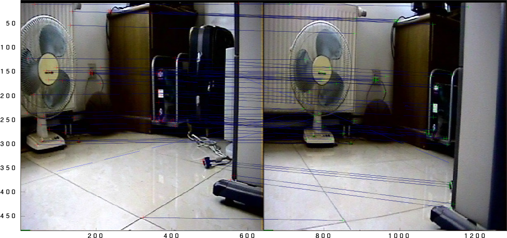
The key-points that are selected by dominant Hue-SIFT yield better matches than classical SIFT features. Each false match is indicated by a blue dotted line connecting two interest points. Their classical SIFT feature vector cannot meet the criterion of a dominant Hue-SIFT feature. All the correctly matched features start at red “+” signs and end where the green “+” signs are located.

3.2. Dimension Reduction

Indexing a complex high-dimensional description vector from a large database creates a heavy computational burden. So the technique of dimension reduction is an essential step in a high-dimensional Hue-SIFT feature space. Principal Component Analysis (PCA), for example, is a popular trick for dimension reduction. The aim of implementing PCA is to achieve dimensionality reduction with a minimum loss of discriminate information. At the same time, we can carry out PCA procedures to reduce the correlation between variables. This also has additional desirable advantages in that it can partly overcome the shortcomings of the following unsupervised learning algorithm.

3.3. Unsupervised Learning

In the field of vision feature based robot localization, we could consider the detected feature vectors in the reference images as sample points in a high-dimensional vector space, and view each query feature vector as a random variable $\mathrm{x}\text{}$ . Then we divide the image retrieval task into several sub-tasks which search each local feature vector detected from the query image. The model images belonging to the same place have many common, similar or even identical interest points, as shown in Fig. 6 and Fig. 7. So there are many repetitive matched features and measures can be taken to reduce the computational burden. It is natural to father those similar feature vectors together to improve the nearest neighbour retrieval tasks. This leads to clustering based on feature similarity. However, there is the problem of how to determine manually the number of clusters in advance.

In general, since we do not really know anything about the compactness, shape or the density of the clusters, determining the appropriate number of prototypes is a difficult task. L. Xu proposed the Rival Penalized Competitive Learning (RPCL) algorithm to solve this problem in [16]. RPCL has its own inherent limitations although it has shown many advantages in the context of competitive learning; that is, the parameters and the penalizing rate should be carefully selected. Otherwise, the resultant clusters would not converge into natural classes.

So we adopt the Robust RPCL algorithm [17] to establish the indexing structure of the feature database. All the model views associated with the same place undoubtedly share many repetitive feature vectors. By using a Robust RPCL algorithm to cluster similar features together, we can not only eliminate most of the redundant computational load of the matching, but also reduce the whole size of the feature database. The key idea behind Robust RPCL is to incorporate four strategies into clustering learning: rival penalization, competition, “limited randomness” and agglomeration. For each initial cluster seed that is selected using the “Limited Randomness” trick, not only the winner seed is attracted by each sample, but also the rival (2nd winner) is forced slightly away from it. After the competitive learning and rival penalization steps, we try to agglomerate these neighbour clusters according to the variance of each cluster, until all of the remaining clusters are distinct from each other. Further details of this approach can be found in the reference [17].

A synthetic data set including four Gaussian clusters of various sizes with a variance of 0.1 is shown in Fig. 8. The “ο” signs represent the positions of 6 initial cluster seeds; the “*” signs stand for each updated coordinate; the pentacles indicate the locations of the final cluster centres after the agglomeration operation. The six various colour curves denote the evolving trajectories of the six initial seeds. In this configuration, depicted in Fig. 8, there are two redundant seeds. However, one seed oscillates as the result of under-penalization, which indicates that the penalizing effect on the redundant seeds is not enough. The top-right two prototypes merge into one cluster using the Robust RPCL algorithm. The composite impact of competition and rival penalization on the six initial seeds achieved a balance after 15 learning iterations. In such cases, the resultant seeds do not change with the increasing learning iterations. Thus the number of correct clusters and nearly exactly correct coordinates of four prototypes are correctly attained at the same time. It shows that, the Robust RPCL algorithm can still work even in situations where there are improper parameters for the RPCL, and it is insensitive to the choice of learning iterations, while it is sensitive in the original RPCL algorithm.

Figure 8.

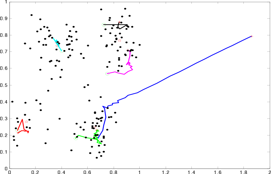
The situation where rival penalization and agglomeration conditions are triggered at the same time. The top-right two similar seeds merge into one group and the blue learning trajectory depicts how this redundant seed is squeezed out.

3.4. Environment Modelling

We can describe the environment model as a group of distinct places and spatial neighbourhood linkages between them. The environment is defined as a topological graph where the nodes and edges are denoted as a collection of places and neighbourhood relationships. Fig. 2 in the second section displays the labels associated with the individual places and the relationships/ transitions between them. Assume that there are $\mathrm{n}\text{}$ locations, we could model the i-th node by using a set of representative images $\left\{{\mathrm{I}}_{\mathrm{j}}^{\mathrm{i}}\right\}\text{}$ and their associated raw and refined Hue-SIFT feature sets $\{{\mathrm{f}}_{\mathrm{k}}({\mathrm{I}}_{\mathrm{j}}^{\mathrm{i}})\}\text{}$ and $\{{\mathrm{f}}_{\mathrm{k}}^{\prime }({\mathrm{I}}_{\mathrm{j}}^{\mathrm{i}})\}\text{}$ . The i-th LFVM is comprised of only those prototype features of interest points belonging to the i-th place after the Robust RPCL learning step and dimension reduction. The LFVM also maintains the links between learned prototype features and their corresponding locations. For a new query image Q and its associated features $\left\{{\mathrm{f}}_{\mathrm{k}}^{\mathrm{Q}}\right\}\text{}$ , after being projected to the eigen-space, a collection of the correspondences between $\left\{{\mathrm{f}}_{\mathrm{k}}^{\mathrm{Q}}\right\}\text{}$ and the model features $\{{\mathrm{f}}_{\mathrm{p}}(\mathrm{i})\}\text{}$ contained in $LPVM(\mathrm{i})\text{}$ is obtained by selecting the nearest neighbour based on the Euclidean distance of the two feature vectors.

4. Bayes Localization

It is quite a challenge for artificial systems to rationally reason with incomplete and uncertain information. We may sometimes make false classifications because of changes in illumination, dynamic environment changes or when the camera pose between the query image and the reference view vary largely. We utilize a probabilistic inference, a Bayes Filter, to tackle observation with large noise, regarding robot localization in the presence of measurements with low resolution.

4.1. Bayes Filter for Localization

The states of a dynamic system are probabilistically estimated from noisy observations by a Bayes Filter. In such cases, the state at time t is denoted by random variables ${\mathrm{x}}_{\mathrm{t}}\text{}$ , the sequence of time-indexed sensor observations about the state is described by ${\mathrm{Z}}^{\mathrm{t}}=({\mathrm{z}}_0,{\mathrm{z}}_1,\cdots ,{\mathrm{z}}_{\mathrm{t}})\text{}$ . At each instance in time, a probability distribution over the state ${\mathrm{x}}_{\mathrm{t}}\text{}$ , called belief, $Bel({\mathrm{x}}_{\mathrm{t}})$ , sequentially estimates the uncertainty of the state ${\mathrm{x}}_{\mathrm{t}}\text{}$ .

Since knowledge of the initial state and all observations ${\mathrm{Z}}^{\mathrm{t}}\text{}$ are obtained up to the current time, it is desirable to estimate the state of the robot at the current time step t when working on robot localization [15]. We can view it as an instance of the Bayes Filter problem, where localization is estimated by computing the belief function $Bel({\mathrm{x}}_{\mathrm{t}})\text{}$ of the current state at all the possible positions in the environment based on all the observations. In [15], the authors treated the places recognized by the Bayes Filter as the prior knowledge with which to facilitate object recognition in the application of wearable computing.

As the robot proceeds, there are two different probabilistic models iteratively used to update the posterior probability $Bel({\mathrm{x}}_{\mathrm{t}})\text{}$ : a system model to incorporate the robot movements $Bel({\mathrm{x}}_{\mathrm{t}})\text{}$ and a measurement likelihood model to update the belief based on the latest sensory input. These two models repeat recursively updating $Bel({\mathrm{x}}_{\mathrm{t}})\text{}$ as below:

(1) Belief Update based on the System Model:

The predictive Probability Density Function (PDF) $\mathrm{P}({\mathrm{x}}_{\mathrm{t}}|{\mathrm{Z}}^{\mathrm{t}-1})\text{}$ is computed to predict the current state of the robot using a system model. The system model here can specifically be defined as the robot motion model, the conditional density $\mathrm{P}({\mathrm{x}}_{\mathrm{t}}|{\mathrm{x}}_{\mathrm{t}-1})\text{}$ , which describes the likelihood of the robot being in position ${\mathrm{x}}_{\mathrm{t}}\text{}$ given the previous position state ${\mathrm{x}}_{\mathrm{t}-1}\text{}$ .

$Be{\mathrm{l}}^{-}({\mathrm{x}}_{\mathrm{t}})=\mathrm{P}({\mathrm{x}}_{\mathrm{t}}|{\mathrm{Z}}^{\mathrm{t}-1})={\displaystyle \int \mathrm{P}({\mathrm{x}}_{\mathrm{t}}|{\mathrm{x}}_{\mathrm{t}-1})}Bel({\mathrm{x}}_{\mathrm{t}-1})\mathrm{d}{\mathrm{x}}_{\mathrm{t}-1}$

(3)

(2)Update Using Current Observation:

The posterior probability density function $\mathrm{P}({\mathrm{x}}_{\mathrm{t}}|{\mathrm{Z}}^{\mathrm{t}})\text{}$ is updated by incorporating the latest observation. The observation likelihood model describes the probability of making such an observation assuming the robot is at the state ${\mathrm{x}}_{\mathrm{t}}\text{}$ .

$Bel({\mathrm{x}}_{\mathrm{t}})=\alpha \mathrm{P}({\mathrm{z}}_{\mathrm{t}}|{\mathrm{x}}_{\mathrm{t}})Be{\mathrm{l}}^{-}({\mathrm{x}}_{\mathrm{t}})$

(4)

where $\alpha \text{}$ is a normalization factor ensuring that $Bel({\mathrm{x}}_{\mathrm{t}})\text{}$ integrates to 1.

The recursive form can be obtained using Eq. 3 and Eq. 4,:

$Bel({\mathrm{x}}_{\mathrm{t}})=\alpha \mathrm{P}({\mathrm{z}}_{\mathrm{t}}|{\mathrm{x}}_{\mathrm{t}}){\displaystyle \int \mathrm{P}({\mathrm{x}}_{\mathrm{t}}|{\mathrm{x}}_{\mathrm{t}-1})}Bel({\mathrm{x}}_{\mathrm{t}-1})\mathrm{d}{\mathrm{x}}_{\mathrm{t}-1}$

(5)

4.2. Topological Localization Using HMM

The State space x is discretized into N locations and the temporal context t is discretized at an appropriate scale. The probabilistic formulation of the localization using image features is to obtain $\mathrm{P}({\mathrm{x}}_{\mathrm{k}}|{\mathrm{f}}_{\mathrm{k}}^{\mathrm{Q}})\text{}$ of each location based on the observation sequence. The procedure determines the likelihood of which node the current acquired view is captured from. If we incorporate the spatial adjacency relationship between the locations, the belief in the recognition will increase significantly. The Hidden Markov Model (HMM), a probabilistic formulation based on a recursive Bayesian Filter, modelling the transition probability between the topological nodes, is applied here to increase the robustness of recognition.

In the general introductions to the HMM, the HMM training is to learn the HMM parameters by using Baum-Welch algorithm. The HMM parameters include the matrix of the transition probability and the matrix of the observation probability associated with each state.

The conditional prior probability is formulated as below:

$\mathrm{P}({\mathrm{x}}_{\mathrm{k}}={\mathrm{x}}_{\mathrm{i}}|{\mathrm{Z}}^{\mathrm{k}-1})={\displaystyle \sum _{\mathrm{j}}^{\mathrm{N}}\mathrm{A}(\mathrm{i},\mathrm{j})\mathrm{P}({\mathrm{x}}_{\mathrm{k}-1}={\mathrm{x}}_{\mathrm{j}}|{\mathrm{Z}}^{\mathrm{k}-1})}$

(6)

Where $\mathrm{A}(\mathrm{i},\mathrm{j})=\mathrm{P}({\mathrm{x}}_{\mathrm{k}}={\mathrm{x}}_{\mathrm{i}}|{\mathrm{x}}_{\mathrm{k}-1}={\mathrm{x}}_{\mathrm{j}})\text{}$ , the transition matrix, means the probability of being at state ${\mathrm{x}}_{\mathrm{i}}\text{}$ based on the state at the immediately previous time step is ${\mathrm{x}}_{\mathrm{j}}\text{}$ . We define $\mathrm{A}(\mathrm{i},\mathrm{j})\text{}$ as inversely proportional to the distance between Location $\mathrm{i}\text{}$ and Location $\mathrm{j}\text{}$ . In the absence of a transition between two locations, the corresponding entry of Matrix $\mathrm{A}\text{}$ was assigned a value of zero. In the final stage all the rows of the matrix were normalized. It illustrates the probability of there being movement between topological nodes and helps to improve the robustness of the recognition.

Here, each individual place associated with several representative images is modelled by a location-relevant LFVM. So each LFVM is comprised of a group of Hue-SIFT prototype features, which are learned by a Robust RPCL of interest points. For a current captured view Q and its associated features, a group of prototype features between Q and LFVM(i) (the model associated with the i-th place), C(Q, LFVM(i)), is computed. The observation likelihood, $\mathrm{p}({\mathrm{z}}_{\mathrm{k}}|{\mathrm{x}}_{\mathrm{k}}={\mathrm{x}}_{\mathrm{i}})\text{}$ , depicts how likely it is that a query view ${\mathrm{Q}}_{\mathrm{k}}\text{}$ at step k is indicated by an ${\mathrm{z}}_{\mathrm{k}}\text{}$ , acquired at the i-th node. This probability can be computed by the ratio of the correspondence set to the total number of matched Hue-SIFT features over the LFVMs of all the locations.

$\mathrm{p}({\mathrm{z}}_{\mathrm{k}}|{\mathrm{x}}_{\mathrm{k}}={\mathrm{x}}_{\mathrm{i}})=\frac{\mathrm{C}(\mathrm{Q},LFVM(\mathrm{i}))}{{\displaystyle {\sum }_{\mathrm{j}}\mathrm{C}(\mathrm{Q},LFVM(\mathrm{j}))}}$

(7)

where $\mathrm{C}(\mathrm{Q},LFVM(\mathrm{i}))\text{}$ characterizes the number of matched modified Hue-SIFT features among the query view and prototype features in the i-th database LFVM(i).

5. Experimental Results and Discussions

5.1. Configurations

The location recognition system allows for topological navigation in large scale complicated environments. Various experiments were carried out to demonstrate the effectiveness of the presented algorithm. The robot system eventually builds a graph-like environment representation where the nodes of the graph correspond to the function-units (in this case, lifts, corridors, offices in one building and so on), whereas the edges of the graph indicate the paths connecting the nodes in indoor environments. We try the first experiment (named Experiment A in Table 1) within a large office environment. The training images are divided into 19 places, as shown in Fig. 3. The training sets are built with six views per place. All the rest of the images are utilized as testing samples.

Table 1.

Comparisons of recognition rates of different features by voting scheme

Recognition Rate	SIFT	SURF	GLOH	RGB SIFT	Hue-SIFT
Experiment A	56.4%	54%	57%	68%	69%
Experiment B	65%	62%	66%	74%	74%
Experiment C	67%	65%	69%	74%	74.6%

Five more indoor location recognition experiments (denoted as Experiment B, C, D, E, F, respectively) are conducted in five different office buildings. We re-trained the Location Feature Vocabulary Model, which is annotated with each individual place using views captured at an interval of 2m. We learn the representative vocabularies associated with those locations from interest point features. The query views are captured randomly along different trajectories under various lighting conditions, dynamic changes of the environments, including wall posters, furniture changes and the presence of people walking.

All the tests are conducted on a robot equipped with a 1.83 GHz laptop (1G memory). The image captured by the monocular camera is 640×480 pixels. In each localization, it took about 135 ms to detect interest points and extract the features (modified Hue-SIFT in this case) in the captured images and 85 ms second to find the correspondent location in the reduced database, which contains only a smaller number of distinct prototype feature descriptors. Another 15 ms is spent on the probability computation. Currently, the proposed algorithm can recognize more than four frames per second without optimization.

5.2. Feature comparisons

To show the effectiveness of the proposed prototype Hue-SIFT feature, we firstly compared the proposed descriptors （dominant Hue-SIFT）with several state-of-the-art descriptors including SIFT [10], colour SIFT (RGB SIFT, here) [21], GLOH [11] and SURF [19]. This approach is tested with three different video sequences per office environment. The average Recognition Rates in three environments are reported in Table 1.

From the results shown in Table 1, it can be seen that the proposed dominant Hue-SIFT and RGB-SIFT always perform the best due to the fact that they have more discriminative power benefiting from colour information and the discriminative feature (here the popular SIFT descriptor). The proposed dominant Hue-SIFT significantly outperforms the original SIFT, with improvements from 7.6% to 12.6%, proving the importance of the dominant hue within a patch in addition to the local discriminative feature. So, those matches similar in local structure but different in hue are considered as false SIFT matches and are rejected. Fig. 7 in sub-section 3.1 shows examples of which Hue-SIFT features yield correct matches while some standard SIFT features give wrong decisions.

The dominant Hue-SIFT is slightly better than the RGB-SIFT in those tests, since we have dropped those interest points the saturation of which is below 0.2 and the intensity of which is below 0.1, or above 0.9, during the traverse stage and the building of the database stage. Thus, the dominant hues play more stable roles than the RGB colour space.

Usually, the Gradient Location-Orientation Histogram (GLOH) descriptor performs better than the SIFT since it uses log-polar bins instead of square bins to compute orientation histograms using SIFT. However, little performance gain has been observed in our tests. In our opinion, this is due to seldom large rotations-in-plane in the video sequences captured by the wheeled robot.

It also can be seen that under circumstances of intentional changes in lighting conditions, back-ground clutter, the dominant Hue-SIFT always performs best among the above features, consistent with their strong properties of illumination invariance and scale invariance.

5.3. Schema comparisons

Next, based on the proposed dominant Hue-SIFT features, we developed three methods and evaluate them in six different teaching building environments, with three different video sequences in each environment. The results are listed in Table 2, where the three methods are indicated as “Hue-SIFT”, “LFVM+voting” and “LFVM+HMM”. The “Hue-SIFT” method is to handle location recognition as an image retrieval problem, representing each location based on the dominant Hue-SIFT features in terms of the model views. The “LFVM+ voting” method represents each location using the LFVM, the database containing the learned discriminative prototypes from the dominant Hue-SIFT features. The location is determined by the LFVM the prototypes of which were frequently classified as matching. The “LFVM+HMM” approach exploited the temporal context by examining the spatial relationships between the locations.

Table 2.

Comparisons of the recognition rates

Recognition Rate	Hue-SIFT	LFVM+ voting	LFVM+HMM
Experiment A	69%	87%	94%
Experiment B	74%	89%	95%
Experiment C	74.6%	90.2%	98.6%
Experiment D	72.6%	88.7%	95.2%
Experiment E	68.7%	85.8%	92.4%
Experiment F	65.2%	75.5%	91%

In the voting scheme, the location that wins the highest number of matched interest points against the query view is considered to be the correct place. Each view in the image sequence acquired by the walking robot is labelled with the index of the corresponding LFVM. From Table 2, it can be seen that the proposed LFVM based on the Hue-SIFT feature is more discriminative than the standard SIFT feature and is very effective.

It has been shown that using colour cues and local textures can eliminate a large number of wrong matches. Moreover, it is very beneficial to associate images from distinct view angles with the same node label.

However, when the voting scheme is used by itself, the two lift-lobbies which share very similar appearances cannot be discriminated clearly. Even for human-beings, without prior context information, distinguishing one such lobby from another is difficult. The second reason for recognition failure is the shortcomings of the local feature descriptions in the application of scenery recognition. The robot itself cannot determine whether the key points belong to the specific furniture, people walking around or places. Only those location-specific key points are helpful in recognizing certain locations, while two other kinds of features belonging to specific furniture or pedestrians may not appear in the query views. For example, there is no poster on the board or the chair may be different between the query and the training samples.

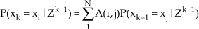
As can be seen in the last column in Table 2, using HMM improved the recognition rate over the voting scheme from 5.5% to 8.4%. The recognition result of the 1st training sequence case using the voting scheme and HMM are shown in Fig. 9, respectively. The recognition rates using the HMM strategy show a better performance than the voting scheme. The HMM, which incorporates all the observation cues contained in an image sequence, performs better than the voting scheme using the current image alone. The transition probabilities between the individual locations modelled by the HMM can increase the robustness of topological localization, reducing wrong decisions. It is obvious that if a robot using just image features gets lost, the probability of it having stayed at its previous location or its immediate neighbourhood and connected location the in topological graph will be much higher than those places far away or inaccessible. We can determine the route/trajectory of the robot from Fig. 9. The observed reality is that it crossed from office 901 (indicated by node 1 in Fig. 2), then it reached room 904 (indicated by node 3 in Fig. 2) across the corridor, and finally, it ended in room 905 (indicated by node 5 in Fig. 2).

Figure 9.

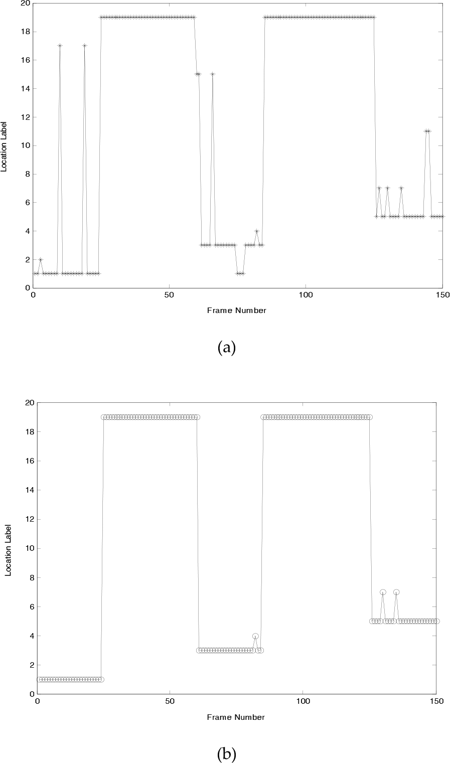
(a) Localization result using voting scheme; (b) Localization result using HMM

When the query image does not directly overlap with the previously learned views, if we apply the voting method without the HMM, there are few features that can be retrieved from those location models, making the probability of the places being an even distribution higher. This therefore causes a loss of confidence until the captured image is able to cover a previously trained location.

Although most video sequences have large deviations from the path of the original exploration trajectories and some lighting conditions change in the environments, the HMM can eliminate previous classification errors and achieve a recognition rate of over 91%. The advantage lies in that the HMM uses recursive probability inference to incorporate the temporal context, which can be modelled by the transition probability matrix. Hence, even when some individual views were misclassified, the robot visiting order during the test trajectory can be determined correctly.

6. Conclusions and discussions

In this paper, we have described a method to estimate the position of a robot with regard to a topological map. We proposed a joint feature that is a combination of colour cues and local textures. In the training/exploration stage, each individual place was modelled by a LFVM, which was constructed based on the Robust RPCL learning procedures. The HMM scheme, not only incorporates the temple order of navigation cues and the spatial context, but also recursively updates the posterior probability using all the available novel features, can increase the robustness of topological localization and can eliminate wrong decisions.

In the results, the modified Hue-SIFT features are implemented for the experimentation but not for the final application. Actually, any kind of local detector and local distinct feature, including the above mentioned SURF, LBP and GLOH, can be incorporated into this localization framework, with differing computational load and accuracy rates. We also tested using Harris corners and found with these it could be greatly faster without a loss of accuracy. The point detector type (using SIFT detector or Harris corner detector) does not have any influence on the accuracy of the proposed method.

The presented method only applied local features to find the most likely qualitative global localization in terms of individual locations. We are developing approaches to combine more cues to increase the recognition rate and conduct precise pose estimations and continuous tracking, which are obtained based on the results of topological localization.