Multi-Focus Image Fusion Using the Local Fractal Dimension

Abstract

Abstract With the development of sensor and image-processing technology, image fusion has become a promising research field. Multi-focus image fusion is an important issue in multi-sensor image fusion. To make full use of the texture features of an image and take into account the inherent advantages of fractal theory in multi-focus image fusion, a new image fusion algorithm using the local fractal dimension (LFD) is proposed. The algorithm first calculates the LFD of each source image pixel-wise by using a blanket method and generates LFD maps of the source images. Then the local energy of each LFD is calculated to generate a decision map, in order to decide pixels of the fused image are from which source image. Finally, the fused image is reconstructed from the source images according to the decision map. Experimental results show that the proposed algorithm outperforms classic LP-based and DWT-based methods according to both visual and objective evaluations.

1. Introduction

With the rapid development of sensor technology, sensors are increasingly used in various fields. An important problem is how to effectively combine the information from different sensors into a single composite for interpretation [1,2]. Thus, sensor fusion is an active research field.

In image-based applications, image fusion is an important branch of multi-sensor fusion. It yields a more precise, comprehensive and robust image representation by combining images from multiple sensors. The fused image is then more suitable for human and machine visual characteristics, and more conducive to further analysis, object recognition and understanding. Thus, image fusion is increasingly important in many fields.

Multi-focus image fusion is an important issue in this field. Camera quality and different camera–object distances limit lenses to focusing only on one object in general. When there are multiple objects in a scene, the object in focus is clear while other objects are indistinct. However, multi-focus image fusion technology can fuse source images focused on different objects to generate an image in which all the objects are in focus [3,4], thereby compensating for camera deficiencies.

The simplest multi-focus image fusion method takes a pixel-wise grey-level average or weighted average of the source images [5]. However, this method often leads to undesirable side effects such as reduced contrast [6,7]. In recent years, multi-scale transform methods have been proposed to address this issue. These methods involve multi-scale decomposition for each source image and all the decomposition coefficients are integrated to form a composite representation. The fused image is finally reconstructed by performing an inverse multi-scale transform [8]. Classic examples of this type of method include the Laplacian pyramid (LP) [9], discrete wavelet (DWT) [10], contourlet transform (CT) [11] and nonsubsampled contourlet transform (NSCT) [12]. However, images fused in this way may still lose some source image information because of the inverse multi-scale transform.

We propose an effective algorithm based on the local fractal dimension (LFD) in the spatial domain that is suitable for multi-focus image fusion. The LFD of each source image is calculated pixel-wise. Then the local energy of each LFD is computed and a decision map is generated by comparing the local energy of each LFD for the source images. Pixels selected from the source images are finally fused according to the decision map.

The proposed algorithm introduces fractal theory into image fusion. By using the LFD in the spatial domain, image texture characteristics such as roughness are utilized and can result in more comprehensive and scientific consideration of image information in the fusion process. Experimental results demonstrate the effectiveness and superiority of the proposed algorithm.

Image registration is an important preprocessing step in image fusion whereby corresponding pixel positions in the source images must refer to the same location. In this paper, we focus on the fusion issue. It is assumed that the source images have already been registered.

The remainder of the paper is organized as follows. Section 2 gives an overview of the fractal dimension (FD). Section 3 addresses the FD in multi-focus images. In Section 4, the proposed fusion scheme is discussed in detail. Section 5 presents and discusses the experimental results. Section 6 concludes.

2. FD Estimation

Texture is an important element of image analysis and processing. Image FD is not only a measure of the complexity of image surface irregularities, but is also invariant for changes in resolution and scale. It is consistent with human visual perception of the roughness of an image surface. The greater the FD of an image, the rougher the image surface, and vice versa.

After Mandelbrot defined the roughness of fractal objects in [13], several approaches for estimating the FD in an image were developed. For example, the ε-blanket method, a 2D generalization of the original approach suggested by Mandelbrot, was proposed by Peleg et al. [14]. Pentland considered the image intensity surface as fractal Brownian function (fBf) and estimated FD from the Fourier power spectrum of fBf [15]. Gangepain and Roques-Carmes [16] and Keller et al. [17] used variations of the box counting (BC) approach to estimate FD. The methods of Peleg et al. and Pentland give accurate results. Thus, we used the blanket method to estimate image FD in this study.

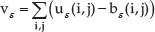
In the blanket method, an image is observed as a relief surface in which heights are proportional to grey levels [14]. All points at distance ε from both sides of the image surface constitute a blanket of thickness 2ε. The covering blanket is defined by its upper surface uε and its lower surface bε. The surface area of the blanket for different ε values can be repeatedly calculated. First, the grey-level value g(i,j) is given for pixel (i,j) and we set u₀(i,j) = b₀(i,j) = g(i,j). The blanket surfaces are defined as follows:

${\mathrm{u}}_{\epsilon }(\mathrm{i},\mathrm{j})=\max \left\{{\mathrm{u}}_{\epsilon -1}(\mathrm{i},\mathrm{j})+1,\underset{\left|\mathrm{d}\{(\mathrm{m},\mathrm{n}),(\mathrm{i},\mathrm{j})\}\right|\le 1}{\max }{\mathrm{u}}_{\epsilon -1}(\mathrm{m},\mathrm{n})\right\}$

(1)

and

${\mathrm{b}}_{\epsilon }(\mathrm{i},\mathrm{j})=\min \left\{{\mathrm{b}}_{\epsilon -1}(\mathrm{i},\mathrm{j})-1,\underset{\left|\mathrm{d}\{(\mathrm{m},\mathrm{n}),(\mathrm{i},\mathrm{j})\}\right|\le 1}{\min }{\mathrm{b}}_{\epsilon -1}(\mathrm{m},\mathrm{n})\right\},$

(2)

where d{(i,j),(m,n)} is the distance between pixels (i,j) and (m,n). The volume of the blanket is then computed as:

${\mathrm{v}}_{\epsilon }={\displaystyle \sum _{\mathrm{i},\mathrm{j}}\left({\mathrm{u}}_{\epsilon }(\mathrm{i},\mathrm{j})-{\mathrm{b}}_{\epsilon }(\mathrm{i},\mathrm{j})\right)}$

(3)

and the surface area as:

$\mathrm{A}(\epsilon )=\frac{{\mathrm{v}}_{\epsilon }-{\mathrm{v}}_{\epsilon -1}}{2}$

(4)

Mandelbrot defined a fractal surface area in [13] as:

$\mathrm{A}(\epsilon )=\mathrm{F}{\epsilon }^{2-\mathrm{D}},$

(5)

where F is a constant and D is the FD of the image. The FD value can be estimated from a linear fit of log{A(ε)} versus log{ε} with a blanket scale from 1 to ε; the slope should be equal to 2-D.

3. FD in Multi-focus Images

For image processing, FD is an important feature for measuring image roughness. In multi-focus images, if an object is in focus, it looks much clear and its grey surface is much rougher. Conversely, if this object is out of focus, it looks blurry and its grey surface is much smoother. Therefore, FD is an indirect measure of image clarity.

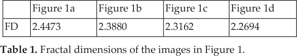
Figure 1 shows an original Lena image and its degraded versions blurred with windows of different sizes. The image FD values are given in Table 1. It is evident that FD decreases with clarity. Another experiment produced similar results, as shown in Figure 2 and Table 2.

Table 1.

Fractal dimensions of the images in Figure 1.

	Figure 1a	Figure 1b	Figure 1c	Figure 1d
FD	2.4473	2.3880	2.3162	2.2694

Table 2.

Fractal dimensions of the images in Figure 2.

	Figure 2a	Figure 2b	Figure 2c	Figure 2d
FD	2.4868	2.3425	2.2352	2.1917

Figure 1.

(a) Original Lena image and degraded versions for blurring windows of (b) w=3, (c) w=7 and (d) w=11.

Figure 2.

(a) Original space image and degraded versions for blurring windows of (b) w=3, (c) w=7 and (d) w=11.

To describe the role of FD in multi-focus images, a set of multi-focus images was further analysed. Two blocks of 64×64 in size were extracted from focused and non-focused areas of an image with the focus on the right of the image. Similarly, two blocks of the same size and position were extracted from the image with the focus on the left of the image. This yielded two sets of blocks for the same positions which were focused and non-focused.

Figure 3 shows the multi-focus images and the blocks extracted from them. FD values were calculated for the blocks and are shown in Table 3. FD is greater for image blocks from the focused compared to the non-focused area. Therefore, in multi-focus images, we can distinguish the source (focused or non-focused) of image blocks or pixels at the same position according to FD. This can be applied in multi-focus image fusion.

Figure 3.

Multi-focus images and extracted blocks: (a) focus on the right; (b) focus on the left; (c) block extracted from a non-focus area of image (a); (d) block extracted from a focused area of image (a); (e) block extracted from a focused area of image (b); (f) block extracted from a non-focused area of image (b).

Table 3.

Fractal dimensions of the images in Figure 3.

	Figure 3c	Figure 3d	Figure 3e	Figure 3f
FD	2.4421	2.6254	2.5413	2.4325

4. LFD-based Multi-focus Image Fusion

Figure 4 shows the proposed multi-focus image fusion algorithm. We consider only two multi-focus source images for simplicity, but this can be extended to more than two images. The fusion algorithm consists of the following steps:

Figure 4.

Schematic diagram of the proposed image fusion method.

• Step 1. Calculate LFD pixel-wise for source images A and B. Let LFD_A(i,j) and LFD_B(i,j) denote the LFD of A(i,j) and B(i,j), where (i,j) is the current pixel position in the source image.

• Step 2. Compare the local energy of LFD_A(i,j) and LFD_B(i,j) and generate the decision map.

• Step 3. Reconstruct the fused image according to the decision map by combining pixels from the source images.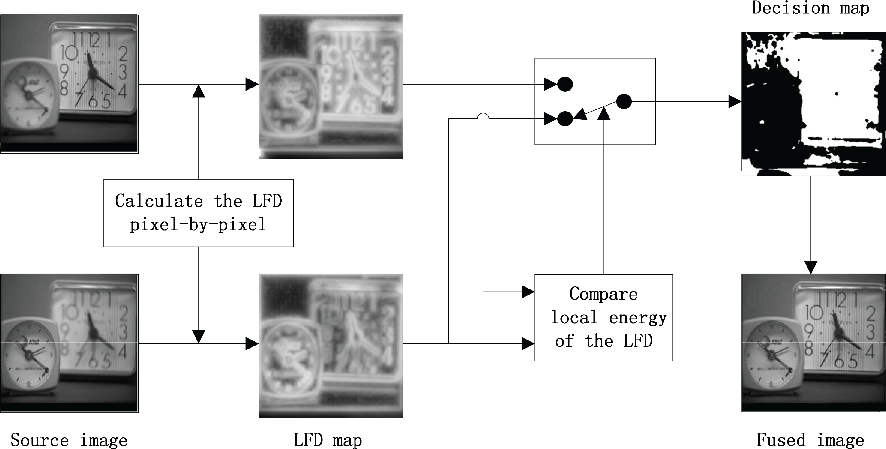

LFD estimation for the source images and the fusion procedure are the most important parts of the proposed algorithm. We now discuss these in depth.

4.1 LFD Estimation

Estimation of global fractal dimension (GFD) has already been reviewed in Section 2, where GFD is the fractal dimension of the whole image. However, in the proposed fusion algorithm, we need the LFD of each pixel in the image instead of GFD. This differs from GFD estimation, which considers the whole image; LFD calculation only considers pixels within a local window centred on the current pixel. The calculation is slightly different between LFD and GFD. First, the grey level value g(i,j) for pixel (i,j) in an image is obtained; we also set u₀(i,j) = b₀(i,j) = g(i,j). Then the surfaces of the blanket are defined as follows:

${\mathrm{u}}_{\epsilon }(\mathrm{i},\mathrm{j})=\max \left\{{\mathrm{u}}_{\epsilon -1}(\mathrm{i},\mathrm{j})+1,\underset{\left|\mathrm{d}\{(\mathrm{m},\mathrm{n}),(\mathrm{i},\mathrm{j})\}\right|\le 1}{\max }{\mathrm{u}}_{\epsilon -1}(\mathrm{m},\mathrm{n})\right\}$

(6)

and

${\mathrm{b}}_{\epsilon }(\mathrm{i},\mathrm{j})=\min \left\{{\mathrm{b}}_{\epsilon -1}(\mathrm{i},\mathrm{j})-1,\underset{\left|\mathrm{d}\{(\mathrm{m},\mathrm{n}),(\mathrm{i},\mathrm{j})\}\right|\le 1}{\min }{\mathrm{b}}_{\epsilon -1}(\mathrm{m},\mathrm{n})\right\}$

(7)

where d{(i,j),(m,n)} is the distance between pixels (i,j) and (m,n), and uε and bε are the top and bottom blanket surfaces, respectively. The volume of the blanket for pixel (i,j) is computed as:

${\mathrm{v}}_{\epsilon }(\mathrm{i},\mathrm{j})={\displaystyle \sum _{(\mathrm{m},\mathrm{n})\in \mathrm{N}(\mathrm{i},\mathrm{j})}\left({\mathrm{u}}_{\epsilon }(\mathrm{m},\mathrm{n})-{\mathrm{b}}_{\epsilon }(\mathrm{m},\mathrm{n})\right)},$

(8)

where N(i,j) denotes a neighbourhood window centred on pixel (i,j). The surface area of pixel (i,j) is:

${\mathrm{A}}_{\epsilon }(\mathrm{i},\mathrm{j})=\frac{{\mathrm{v}}_{\epsilon }(\mathrm{i},\mathrm{j})}{2\epsilon }.$

(9)

On the other hand, the area of a fractal surface is [13]:

${\mathrm{A}}_{\epsilon }(\mathrm{i},\mathrm{j})=\mathrm{F}{\epsilon }^{2-\mathrm{D}}$

(10)

where F is a constant and D is the FD of pixel (i,j). Therefore, FD can be obtained from the slope of a linear plot of A_ε(i,j) versus ε on a log-log scale for a blanket scale from 1 to ε; the slope should be equal to 2-D. Then we obtain the LFD of an image when the FD values for all pixels are calculated.

The actual log-log plot of the blanket area A(ε) versus ε is a non-linear curve. This is especially true for a small window. Thus, the LFD value largely depends on the size of ε, which needs to be optimized for more precise LFD. The LFD map is generated by calculating LFD using the optimized ε.

4.2 Image Fusion Based on LFD

In this subsection the fusion procedure based on LFD maps of source images is discussed in detail. Grey-level matrixes for source images A and B are denoted by G_A and G_B, and their LFD maps are denoted by LFD_A and LFD_B, respectively. The decision map generated from these is denoted by D_F.

The simplest pixel-based fusion rule generates the decision map by comparing the LFDs of corresponding pixels of source images directly, as below:

${\mathrm{D}}_{\mathrm{F}}(\mathrm{i},\mathrm{j})=\{\begin{array}{c}1,\mathrm{\dots ..}if\mathrm{..}LF{\mathrm{D}}_{\mathrm{A}}(\mathrm{i},\mathrm{j})\ge LF{\mathrm{D}}_{\mathrm{B}}(\mathrm{i},\mathrm{j})\\ 0,\mathrm{\dots ..}if\mathrm{..}LF{\mathrm{D}}_{\mathrm{A}}(\mathrm{i},\mathrm{j})<LF{\mathrm{D}}_{\mathrm{A}}(\mathrm{i},\mathrm{j})\end{array},$

(11)

However, this pixel-based rule is very sensitive to noise and has poor robustness since it only considers the current pixel and ignores all other pixels. Therefore, a window-based fusion rule was applied to generate the decision map. This rule first identifies the LFD values in each LFD map. The importance of LFD(i,j) is determined according to the local energy, denoted by EoD(i,j) and calculated for a window centred on pixel (i,j):

$EoD(\mathrm{i},\mathrm{j})={\displaystyle \sum _{(\mathrm{m},\mathrm{n})\in \mathrm{N}(\mathrm{i},\mathrm{j})}LFD{(\mathrm{m},\mathrm{n})}^2},$

(12)

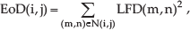
where N(i, j) denotes the neighbourhood window centred on the LFD value of pixel (i,j). Typically, the window size is 3×3 or 5×5.

Local energy values for corresponding positions in the two LFD maps are compared to decide which source image should be used to construct the fused image. Here, pixels in the source images with greater local energy were chosen to reconstruct the fused image. In the decision map, a value of 1 indicates that a pixel is from source image A, similarly, 0 indicates source image B. This process is defined as:

$\mathrm{D}(\mathrm{i},\mathrm{j})=\{\begin{array}{c}1,\mathrm{\dots ..}if\mathrm{..}Eo{\mathrm{D}}_{\mathrm{A}}(\mathrm{i},\mathrm{j})\ge Eo{\mathrm{D}}_{\mathrm{B}}(\mathrm{i},\mathrm{j})\\ 0,\mathrm{\dots ..}if\mathrm{..}Eo{\mathrm{D}}_{\mathrm{A}}(\mathrm{i},\mathrm{j})<Eo{\mathrm{D}}_{\mathrm{B}}(\mathrm{i},\mathrm{j})\end{array}.$

(13)

Then all the pixels selected are merged to reconstruct the fused image according to the decision map:

$\mathrm{F}(\mathrm{i},\mathrm{j})=\{\begin{array}{c}{\mathrm{G}}_{\mathrm{A}}(\mathrm{i},\mathrm{j}),\mathrm{\dots ..}if\mathrm{..}\mathrm{D}(\mathrm{i},\mathrm{j})=1\\ {\mathrm{G}}_{\mathrm{B}}(\mathrm{i},\mathrm{j}),\mathrm{\dots ..}if\mathrm{..}\mathrm{D}(\mathrm{i},\mathrm{j})=0\end{array}.$

(14)

The fusion result then needs to be verified and corrected. Specifically, if the centre pixel comes from source image A but the majority of its surrounding pixels are from source image B, then we change this centre pixel to be from source image B, and vice versa. A filter with a 3×3 window was used for this step.

5. Experimental Results

5.1 Optimization of the Number of Blankets

Previous results demonstrated that a local window of 3×3 is suitable for extracting local features from images [18]. Thus, we used a local window of 3×3 and only the size of ε needs to be optimized.

The method for calculating LFD was extended from GFD estimation. Therefore, the ε size used to estimate GFD was applied to calculate LFD. We investigated the behaviour of GFD for a range of ε values to optimize ε. To facilitate comparisons, GFD values were normalized to a range of 0–1.

Figure 5 shows the GFD behaviour for multi-focus clock images (Figures 6(a) and (b)) for ε=80−160. It can be seen from the diagram that the values of GFD reach the maximum respectively when ε=130 and ε=150 in multifocus ‘clock’ images. In order to obtain a more precise fused result, we use the same size of ε to calculate the LFD for different source images in multi-focus image fusion procedure. For example, the LFDs of Figures 6(a) and (b) are calculated with ε=140, which is the value at the intersection of two curves in Figure 5. In later fusion experiments, this approach is used to estimate the size of ε to calculate the LFDs of multi-focus images.

Figure 5.

Estimated GFD for multi-focus clock images vs. ε.

Figure 6.

Multi-focus clock images and their LFD maps.

In the LFD map, the value at each position (i,j) is the LFD value estimated from a 3×3 local window centred at (i,j) in the original image. To facilitate observations, the LFD map was generated by transforming LFD values to the range 0–255 instead of the typical range of 2.0–3.0. Figures 6(a) and (b) are original multi-focus images of 256×256 pixels with 256 grey levels. The corresponding LFD maps are shown in Figures 6(c) and (d), respectively. It is evident from the LFD maps that greater brightness corresponds to a greater LFD value.

5.2 Fusion Results

The multi-focus images shown in Figures 10 and 11 were used to compare the proposed algorithm with algorithms based on LP and DWT transforms. In Figures 10(a) and (b) the focus is on the Pepsi can and the test card, respectively. In Figures 11(a) and (b) the focus is on the bookshelf and the clock, respectively. The source images used in experiments all had a grey level of 256 and were 256×256 in size for Figure 10 and 240×320 for Figure 11.

Figure 7.

Estimated GFD for multi-focus Pepsi images vs. ε.

Figure 8.

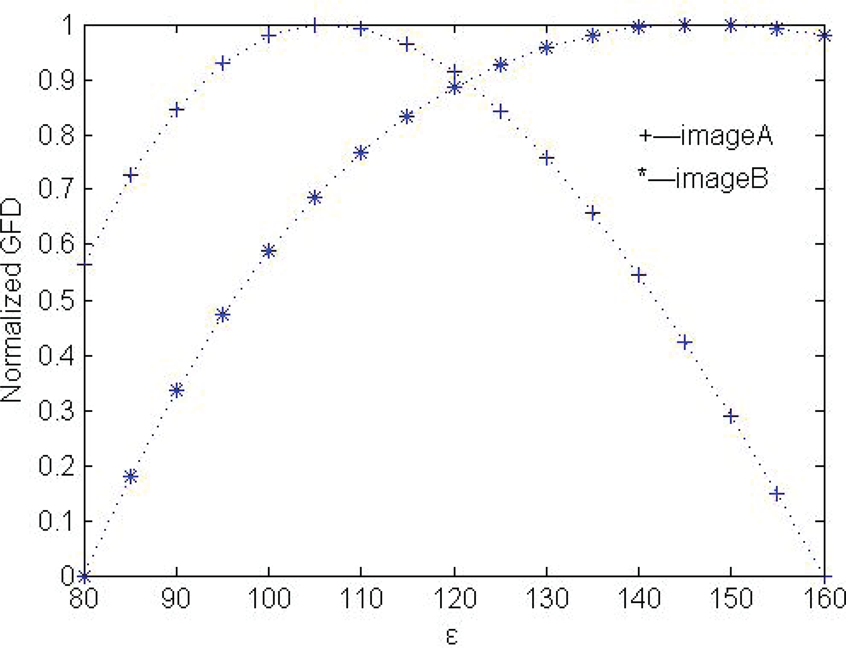
Estimated GFD for multi-focus disk images vs. ε.

Figure 9.

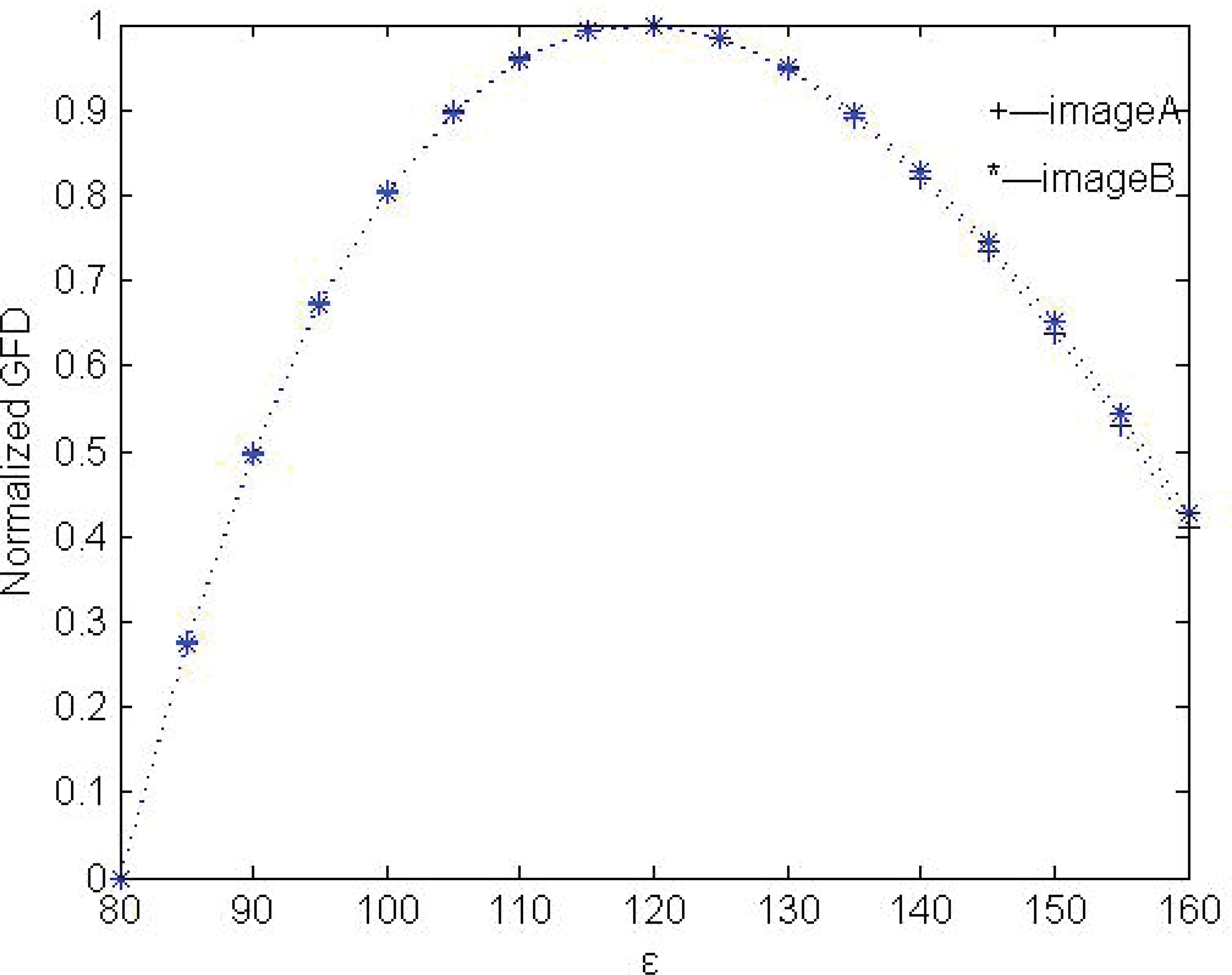
Estimated GFD for multi-focus artificial images vs. ε.

Figure 10.

Experimental results for Pepsi images with focus on (a) the Pepsi can and (b) the test card. (c) LFD map of (a). (d) LFD map of (b). (e) Decision map. (f) LP-based fusion result. (g) DWT-based fusion result. (h) Result for the proposed method. (i) Difference between (f) and (a). (j) Difference between (g) and (a). (k) Difference between (h) and (a). (l) Difference between (f) and (b). (m) Difference between (g) and (b). (n) Difference between (h) and (b).

Figure 11.

Experimental results for disk images with a focus on (a) the clock and (b) the books. (c) LFD map of (a). (d) LFD map of (b). (e) Decision map. (f) LP-based fusion result. (g) DWT-based fusion result. (h) Result for the proposed method. (i) Difference between (f) and (a). (j) Difference between (g) and (a). (k) Difference between (h) and (a). (l) Difference between (f) and (b). (m) Difference between (g) and (b). (n) Difference between (h) and (b).

For the LP-based and DWT-based fusion methods, a decomposition level of 3 was used. The lowpass subband coefficients were merged using an average scheme and the bandpass subband coefficients were merged using an ‘absolute maximum choosing’ scheme. The dbss(2,2) wavelet was used in the DWT-based method. For the proposed algorithm, we used ε=120 and ε=130 to estimate the LFD map of the source images in Figures 10 and 11 according to the experimental results shown in Figures 7 and 8, respectively.

Experimental fusion results for the proposed method and the comparison methods are given in Figures 10 and 11. Figures 10(c) and (d) are the LFD maps of source images (a) and (b) respectively. Figure 10(e) is the decision map, which can decide which source image should be used to construct the fused image. From the decision map, we can see that pixels from the focused area are selected correctly. Figures 10(f), (g) and (h) show fused results using the LP-based, the DWT-based and the proposed method, respectively. For ease of comparison, the differences in images between the fused images and the source images are given in Figures 10(i)–(n); these images make the results from the different methods distinguishable by the human eye. For the focused area, the difference between the fused image and the source image should be zero. For instance, in Figure 10(a) the test card is clear, and in (k) the difference between Figures 10(h) and (a) in the test card region is slight. This demonstrates that the whole focused area is contained in the fused image successfully. However, the difference between Figures 10(f) and (a), and Figure 10(g) and (a) in the test card region shown in Figures 10(i) and (j), are greater. These results show that the proposed method gives better visual results and provides more detailed information than the other two methods. The same conclusion can be obtained from Figure 11.

Another set of artificial multi-focus images of size 256×256 is also used to compare the fusion algorithms, as shown in Figure 12. The multi-focus source images were produced from a reference image by blurring different objects in the scene. ε=120 was used to calculate the LFD according to the experimental results in Figure 9. The difference images between the fused image and the source images are given in Figure 12, showing similar results to the previous examples.

Figure 12.

Experimental results for artificial multi-focus images with a focus on (a) the right and (b) the left. (c) LFD map of (a). (d) LFD map of (b). (e) Decision map. (f) LP-based fusion result. (g) DWT-based fusion result. (h) Result for the proposed method. (i) Difference between (f) and (a). (j) Difference between (g) and (a). (k) Difference between (h) and (a). (l) Difference between (f) and (b). (m) Difference between (g) and (b). (n) Difference between (h) and (b).

For further comparison, three objective criteria were used to evaluate the performance of the fusion algorithms. The first criterion is spatial frequency (SF), which originated from the human visual system and measures the overall activity level of an image. The human visual system is too complex to be fully understood with present physiological means, but SF is an effective objective quality index for image fusion [19].

The second criterion is the Q^AB/F metric. It uses the Sobel edge operator to calculate the strength and orientation information at each pixel in both source and fused images, and considers the amount of edge information transferred from source images to the fusion result [20]. For the ideal situation, Q^AB/F=1.

The third criterion is mutual information (MI). This metric indicates the total amount of information that the fused image F contains from A and B [21]. It is defined as the sum of mutual information between each source image and the fused image:

$\mathrm{M}{\mathrm{I}}_{\mathrm{F}}^{AB}={\mathrm{I}}_{FA}(\mathrm{f},\mathrm{a})+{\mathrm{I}}_{FB}(\mathrm{f},\mathrm{b}),$

(15)

where I_FA(f,a) and I_FB(f,b) denote the mutual information between the fused image and the source images A and B, respectively.

For all three criteria, the larger the measure value, the better the fusion performance.

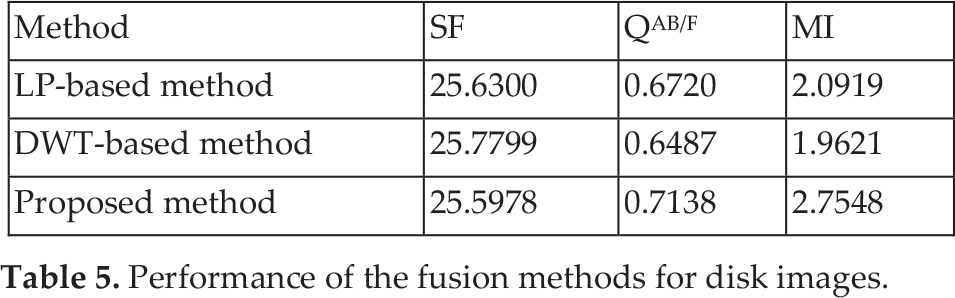
Objective evaluation values for Figures 10, 11 and 12 are listed in Tables 4, 5 and 6, respectively. The SF values are almost the same for the three fusion algorithms. However, the proposed algorithm outperforms the LP-based and DWT-based methods in terms of Q^AB/F and MI. Overall, it provides much better performance than the other two methods.

Table 4.

Performance of the fusion methods for Pepsi images.

Method	SF	QAB/F	MI
LP-based method	19.1224	0.7290	2.3924
DWT-based method	19.1847	0.7003	2.2224
Proposed method	19.1423	0.7494	2.8589

Table 5.

Performance of the fusion methods for disk images.

Method	SF	QAB/F	MI
LP-based method	25.6300	0.6720	2.0919
DWT-based method	25.7799	0.6487	1.9621
Proposed method	25.5978	0.7138	2.7548

Table 6.

Performance of the fusion methods for artificial multifocus images.

Method	SF	QAB/F	MI
LP-based method	41.8965	0.8641	3.6873
DWT-based method	41.9393	0.8541	3.4869
Proposed method	41.9115	0.8753	4.0874

A shortcoming of the proposed algorithm is that it is slightly more time-consuming than LP-based and DWT-based methods for LFD estimation.

6. Conclusion

An LFD-based multi-focus image fusion algorithm implemented in the spatial domain has been proposed in this paper. The algorithm calculates the LFD from a local area for each pixel in source images, and generates LFD maps for these source images. Then the local energy of LFD is computed and a decision map is obtained. Finally, a fused image is constructed from the source images, according to the decision map. As a measure to describe image texture features, fractal dimension can extract texture information of an image effectively. By introducing it into the image fusion procedure, more detailed texture information can be transferred from source images to the fused image. The proposed algorithm is performed furthermore in the spatial domain. It operates pixels directly, and this ensures the fusion results have the further advantage of preserving detailed information. The proposed algorithm was compared to LP-based and DWT-based classic methods. Experimental results show that the proposed algorithm has better performance in terms of both visual quality and objective evaluation.

7. Acknowledgements

This work was supported by the National Basic Research Program of China (973 Program) 2012CB821200 (2012CB821206), the National Natural Science Foundation of China (No. 91024001, No. 61070142) and the Beijing Natural Science Foundation (No. 4111002).