Quantile Acoustic Vectors vs. MFCC Applied to Speaker Verification

Abstract

In this paper we describe speaker and command recognition related experiments, through quantile vectors and Gaussian Mixture Modelling (GMM). Over the past several years GMM and MFCC have become two of the dominant approaches for modelling speaker and speech recognition applications. However, memory and computational costs are important drawbacks, because autonomous systems suffer processing and power consumption constraints; thus, having a good trade-off between accuracy and computational requirements is mandatory. We decided to explore another approach (quantile vectors in several tasks) and a comparison with MFCC was made. Quantile acoustic vectors are proposed for speaker verification and command recognition tasks and the results showed very good recognition efficiency. This method offered a good trade-off between computation times, characteristics vector complexity and overall achieved efficiency.

1. Introduction

There have been several approaches for biometry recognition using an individual's physical characteristics, which can be acquired through signals originated from the human body or specific traits in the individual's physiology. These signals could be used for several purposes, such as pathology detection, biometric identification or autonomous systems applications. Two stages are critical in both cases: 1) the extraction of characteristics and data representation in order to emphasize the attributes that allow recognition and 2) characteristics modelling and model generation, according to their classes. In the human body context, the respiratory system is closely related with the vocal tract (which has been extensively studied) and the sub-glottal areas (a topic of detailed acoustic research as well). The combined effect of both systems gives very distinctive properties to the vocal tract; for instance relatively short wavelengths suggest that useful information in the lung structure could be obtained from acoustic measurements at low frequency ranges [1, 2].

Speech analysis is typically made in a succession of elemental, theoretically stationary segments, which are typically called analysis windows. The principles are sustained in modelling either the vocal tract or the human ear function paradigm and its interpretation in the human brain. In these processes, a spectral analysis is applied each given time over the windows (typically 30ms) with a time shift (typically 20ms, which results in overlapping) in order to generate an acoustic vector for each window.

There are many different technologies in voice signal representation, but we will only discuss a few. Some of them were developed specifically for voice signal compression, while others are widely used in speaker recognition systems. Most of them are Fourier transform-based methods. Another successful approximation is the so-called cepstrum deconvolution. An extension of the cepstral principles and their representation into a logarithmic frequency space, which relates with human audition, is the very successful MFCC vector [3–6]. Another common approximation derived from MFCC vectors is the TFCC coefficients, because unlike the previous MFCC, the frequencies of its filters are uniformly distributed on a linear frequency scale instead of the Mel scale [7].

A very well known method in the voice transmission field and VoIP is Linear Predictive Coding (TPC). This method rests mainly on the hypothesis that the voice can be modelled by a linear predictive process [3, 4, 8].

There exist other methods like PTP, which modify the voice power spectrum before obtaining an approximation by an autoregressive model [9, 10]. Also, there are other variants of this methodology, which are more adapted to communication channels such as RASTA PTP (RelAtive SpecTrAl) [3, 9]. Among other methods that have been applied in recognition systems, we can find the wavelet transformation, in which the signal is comprised of a sum of wavelets [3].

As previously mentioned, human physiology and anatomy influence acoustic measures, hence an adequate representation of an acoustic vector is necessary. Some researchers conducted studies in order to determine the existence of respiratory pathologies [1]; these studies obtained successful measurements which were represented by quantiles, also known as percentiles and such experiments inspired the approach presented here.

2. Quantile Vectors in the Autonomous Systems Context

The automatic speaker verification (ASV) and Speech recognition systems try to take advantage from acoustic and articulatory representations of the speech signal [8, 11–13]. Nevertheless, inter-speaker variability renders the recognition process difficult [14, 15]. Additionally, the variability is influenced by recording and transmission tools [14].

Traditionally, acoustic vectors were not thought to be used in autonomous systems. Speech technology tends to be more and more embedded in mobile phones or other portable communication terminals. Considering low consumption devices, with little memory available to store acoustic models, distant recognition is still interesting, even for tasks like command recognition in robots. Some solutions could be proposed when the spectral analysis can be performed in autonomous systems; one of them is optimizing the computational cost of acoustic vectors [16].

Nowadays, there are devices oriented to help handicapped people [17]; some examples of biomedical researchers' work deals with heart signals, arm aid devices and (less frequently) with voice controlled systems. Introducing speech modules on autonomous systems make these devices more useful and easier to work with.

A system's acoustic model should be optimized in order to build an embedded system, as in the case of a wheelchair controlled by speech commands [18]. To make commands interesting for a general audience, they should be in a conventional language, in order to sound natural and more comprehensible, even for non-scientists. Memory and computational costs are also important, because in autonomous systems there are constraints on command processing and power consumption, so it is mandatory to have a good trade-off between accuracy and computational requirements. To reach a satisfactory level of recognition performance, it is necessary to work with well-trained acoustic models, but at the same time it is necessary to optimize models for autonomous systems [18, 19]. One needs to consider who is going to speak to the system and if there is more than one person that will use it. Sometimes, a good hypothesis is to think of a mono-speaker system such as a robotic wheelchair [18].

An example of a mono-speaker system is a planar robot controlled by a speech commands (PRCSC) system, which maps utterances to a set of control signals used to drive a planar system. Additionally, it allows a small set of discrete spoken words, adaptable/applicable as commands, to set a (x,y)XY position.

Human-machine interfaces can be bi-directional communication systems; but in this work a one-direction approach is enough since typically one person commands the machine through a voice interface. The spoken command recognizer must be robust to users with diction problems and manage the normal variations a given person exhibits in their voice from time to time.

In previous work [18], we carried out experiments to recognize commands and control a planar system. In these experiments, 94.16% recognition accuracy was achieved through Dynamic Time Warping (DTW). Further results were obtained by applying Gaussian Mixture Models (GMM) with eight and 16 Gaussians. Consequently, the optimized GMM model used eight densities and obtained 92.5% recognition accuracy, and was even faster than the DTW method [18]. In both cases, DTW and GMM, MFCC acoustic vectors were applied. This was important in order to take care of the limited resources involved in embedded systems. In an attempt to improve this approach, we decided to apply quantile vectors in command recognition experiments, which will be presented in Section 7 as another front-end alternative. The GMM technique is computationally less expensive than Hidden Markov Models. Tikewise, quantile vectors are computationally less expensive than MFCC [15, 18, 20]. That is why we chose to experiment with quantile vectors and GMM as an alternative to the aforementioned techniques.

3. Quantiles

In statistical theory, non-centralist tendency measurements allow us to know particular aspects in a given distribution and one of the most important is the quantile. In this method the data is sorted from low to high and the resultant distribution function is divided into n parts of equal area. The quantiles define the limit between these consecutive area segments.

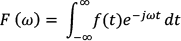
One of the probability axioms states that the total probability area must be equal to one. The quantile q_pq of a given random variable is also defined as the smallest number qq such as its Cumulative Density Function (CDF) is equal or higher that a given value pp, where pp is 0 < p < 10< [21]. This can be calculated for a continuous distribution function using its Probability Density Function f(x), as shown in (1).

$p=\underset{-\mathrm{\infty }}{\overset{q_p}{\int }}f\left(x\right)dx$

(1)

In order to find q_p, the CDF's inverse transform is applied:

$q_p=F^{-1}\left(p\right)$

(1)

Stating it in another way, the pp-th Quantile q_pq of a given random variable X, is the value such that:

$F\left(q_p\right)=P\left(X\le q_p\right)=p\hspace{0.17em}\text{for:}\hspace{0.17em}0<p<1$

(2)

3.1 Octiles

A particular case of quantile is the octile. The octile values identify the area limits that a random variable takes along a given known Probability Density Function (0.125%, 0.25,…0.875%). It is important to note that the last quantile is not of interest because it is always one. The octiles can take the following notation: q_0.125, q_0.25, …, q_0.875, respectively.

The idea was to achieve a simpler acoustic representation than MFCC, while keeping a reasonable computational cost. The purpose of the experiments was to understand the influence of the energy changes and their impact on the frequency components of the signal. Experimentally, this led to the application of octiles.

In the first stage, speech signals uttered by speakers were used (Figure 1). Then, the fast Fourier transform (FFT) was applied, as is depicted in and (3). Complying with the mentioned axiom for the Probability Density Function, the FFT area is normalized to unity (4).

$F\mathrm{\hspace{0.17em}}\left(\omega \right)=\mathrm{\hspace{0.17em}}{\int }_{-\mathrm{\infty }}^{\mathrm{\infty }}f\left(t\right)e^{-j\omega t}dt$

(3)

Figure 1.

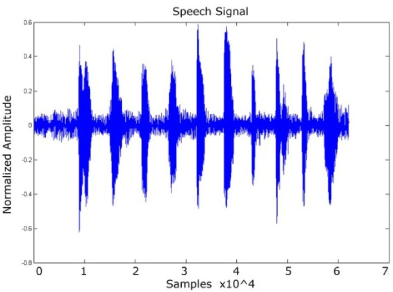
Voice signal, time vs. amplitude, speaker 005, Session 1, phrase 1

Figure 2.

Voice signal, frequency vs. amplitude, speaker 005, Session 1, phrase 1

$F_N\mathrm{\hspace{0.17em}}\left(\omega \right)=\mathrm{\hspace{0.17em}}\frac{{\int }_{-\mathrm{\infty }}^{\mathrm{\infty }}f\left(t\right)e^{-j\omega t}dt}{area(\mathrm{\hspace{0.17em}}F\left(\omega \right)\mathrm{\hspace{0.17em}})}$

(4)

$\begin{array}{c}A=.125={\int }_{-\mathrm{\infty }}^{f_{.125}}{F}_N\left(f\right)\mathrm{\hspace{0.17em}}df\mathrm{\hspace{0.17em}},\dots ,\mathrm{\hspace{0.17em}}A=.875\\ ={\int }_{-\mathrm{\infty }}^{f_{.875}}{F}_N\left(f\right)\mathrm{\hspace{0.17em}}df\end{array}$

(5)

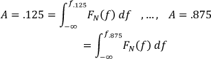
After normalization, it is necessary to analytically compute q_pq, with the CDF's inverse transform (6) and find the values f_0.125, f_0.25, …, f_0.875f, (i-e., each one of the octiles coefficients), but this is not a trivial task. Algorithmically, the octiles were calculated through an iterative sum in order to obtain the q_pq that limits the area segments under F_N (ω), thus detecting the frequency values for q_0.125, q_0.25, …, q_0.875q. Computationally, the quantile coefficients (Mel-scale) in the fixed-point algorithm could be summarized as follows:

Extract wav data and frequency sampling

Compute FFT to obtain the PSD

Apply the logarithm (base10) to the PSD curve and normalize it.

The Mel scale was normalized, so the Q coefficient would correspond to it.

Iterate along the normalized PSD to compute the quantile coefficients Q.

3.2 Parameterization

The experiments were carried out with two representations of an octile vector. In the first one, which will be referred to as long-time, a single octile vector was obtained per recording (always a 1 × 71times7 matrix). In the second one (referred to as short-time), an octile vector was obtained for each frame with 400ms size and a frame shift of 300ms (an overlapping of 100ms), resulting in a n × 7n matrix, where n is the number of frames per recording. In both cases, several audio preprocessing methods were tried, such as pre-emphasis, audio normalization and filtering. Moreover, several experiments were done regarding the signal's energy and amplitude in order to obtain the quantiles. Nevertheless, after many trials, it was decided not to use signal preprocessing in the present work, since our results were overall better with the original, 8 kHz-sampled database.

4. GMM Modelling

This section describes the Gaussian mixture model (GMM) as a pattern recognition paradigm. These models were popularized by Reynolds' work [22, 23] in the speaker identification context. These techniques were already known in the pattern recognition context [24] as powerful methods. Here, GMM is used as a Speaker Verification method.

A class-conditional probability represents the distribution of characteristics probabilities for each class. The a priori probability means our initial degree of belief that an observed characteristics set corresponds to the jj-th class. The process in which these types of probabilities are calculated determines the way to build a model. In our case, the model (Client or Impostor) will be determined by the weighted sums of Gaussian densities (or GMM, from Gaussian Mixture Model), as shown in (6).

$P\left(\overrightarrow{x}|\lambda \right)={\displaystyle \sum _{i=1}^M}{m}_i{b}_i\left(\overrightarrow{x}\right)$

(6)

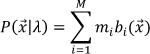
where xx is a d-dimensional random vector (7-dimensional in our octiles vectors case), and b_i(x)b for i = 1,…,Mi= represents the M Gaussian densities used for the model computation, as shown in (7).

$b_i\left(\overrightarrow{x}\right)=\frac{1}{{(2\pi )}^{D/2}{\left|\mathrm{\Sigma }\right|}^{1/2}}exp\left\{-\frac{1}{2}\left(\overrightarrow{x}-{\overrightarrow{\mu }}_i\right){\sum }_i^{-1}(\overrightarrow{x}-{\overrightarrow{\mu }}_i)\right\}$

(7)

µ_iµ and Σ _i Σ represent the mean vector and the covariance matrix, respectively. On the other hand, the mixture weights satisfy the constraint that ${\sum }_{i=1}^M{m}_i$ must be equal to 1. The whole GMM model is parameterized by the mean vectors, covariance matrices and mixture weights from its Gaussian densities. The model that collects the parameters is represented by (8) [22–24].

$\lambda =\left\{m_i,{\overrightarrow{\mu }}_i,{\mathrm{\Sigma }}_{\mathrm{i}}\right\}i=1,\dots ,M$

(8)

For ASV, speaker sets were created and represented as GMM models λλ (Client and Impostor). The verification procedure will be explained in detail in a posterior section.

Expectation-maximization (EM) is a powerful algorithm widely utilized to compute parameters and a very good review of it is found in [20]. In this paper, we just show the main equations. The basic idea is, given the training data, for a sequence of NN training vectors (obtained from uttered phrases by speakers) $X={\left\{{\overrightarrow{x}}_t\right\}}_{t=1}^N$ the GMM likelihood can be written as:

$p(X|\lambda )={\displaystyle \prod _{t=1}^N}p\left({\overrightarrow{x}}_t\right|\lambda )$

(9)

Hence, we need to have an initial model λλ in order to estimate successive models λ, such that:

$p\left(X\right|\stackrel{-}{\lambda })\ge p(X\left|\lambda \right)$

(10)

The new model then becomes the initial model for the next iteration and the process is repeated until some convergence threshold is reached. The parameters must be re-estimated in each EM iteration using the following formulas:

${m_i}^{\text{new}}=\frac{1}{N}{\displaystyle \sum _{t=1}^N}p\left(i\right|{\overrightarrow{x}}_t,\lambda )\hspace{0.17em}$

(11)

${{\mu }_i}^{\text{new}}=\frac{\sum _{t=1}^N{x}_{t}p\left(i\right|{\overrightarrow{x}}_t,\lambda )}{\sum _{t=1}^{N}p\left(i\right|{\overrightarrow{x}}_t,\lambda )}\hspace{0.17em}$

(12)

$\begin{array}{c}{{\sum }_i}^{\text{new}}\hfill \\ =\frac{\sum _{t=1}^{N}p\left(i\right|{\overrightarrow{x}}_t,\lambda )\left({\overrightarrow{x}}_t-{{\mu }_i}^{\text{new}}\right){\left({\overrightarrow{x}}_t-{{\mu }_i}^{\text{new}}\right)}^T}{\sum _{t=1}^{N}p\left(i\right|{\overrightarrow{x}}_t,\lambda )}\hfill \end{array}$

(13)

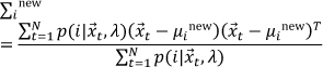
The a posteriori probability for acoustic class ii is given by the following equation:

$p\left(i|{\overrightarrow{x}}_t,\lambda \right)=\frac{m_i{b}_i\left({\overrightarrow{x}}_t\right)}{\sum _{k=1}^M{m}_k{b}_k\left({\overrightarrow{x}}_t\right)}$

(14)

5. Speaker Verification System (SVS) and XM2VTS8K

An SVS system's efficiency depends highly on the quantity of available signals and the training data set size. The system's purpose is to classify acoustic signals by fitting them in one of two classes: Client, which represents a subject we want to identify and Impostor (anyone who claims a false identity), which is any individual who is not part of the client set. Nevertheless, the system may return two types of errors: False Acceptation (FA), when then system classifies an impostor as a client and False Rejection (FR), when the system rejects an actual client. Efficiency is measured by using these errors as measurements.

$\begin{array}{cc}& \begin{array}{c}FAR=\frac{F{A}^{\mathrm{\prime }}s\mathrm{\hspace{0.17em}}quantity}{Total\mathrm{\hspace{0.17em}}Imposter\mathrm{\hspace{0.17em}}trials}\\ FRR=\frac{F{R}^{\mathrm{\prime }}s\mathrm{\hspace{0.17em}}quantity}{Total\mathrm{\hspace{0.17em}}Client\mathrm{\hspace{0.17em}}trials}\end{array}\end{array}$

(15)

The rate (or difference, in the logarithmic domain) of test signals and the client model is compared to a decision threshold. If this measure is above a threshold, the speaker is accepted (assumed to be a client), and rejected otherwise (assumed to be an impostor). This threshold is the allowed tolerance based on system specifications, in our case a range of thresholds was calculated using an evaluation partition. With the aim to compute a satisfactory decision threshold (Δ _i Δ), the system is frequently adjusted over a validation data set. Determining this threshold is critical to assuring the appropriate behaviour of the verification system. If it becomes too high, the False Rejection Rate (FRR) will be very high; on the other hand, if it becomes too low, the False Acceptation Rate (FAR) will become inadmissible. In consequence, the Equal Error Rate (or simply EER) is used; this corresponds to the intersection of the FAR and FRR curves in a given threshold interval. EER is the point in which FAR and FRR have the same value. Since this is not easily achieved given the discrete nature of both curves, the intersection of the curves is computed instead. This is the value in the EER curve in which we are interested, as it represents the system's efficiency verification.

The XM2VTS8K Database has 24 recordings by each Speaker, where all of them are wav files. These files consist of four sessions in which three different and phonetically balanced phrases were recorded twice. It was expected to find 295*4*3*2, but some speakers recording sessions were incomplete, leaving only 7062 recordings.

The implemented Speaker Verification system structure is shown in Figure 3. The acoustic characteristics extracted from the signal are compared with a model corresponding to the claimed client (obtained from the database models previously computed for this purpose) and with another model, which represents the impostor (also previously computed). The rate ΘΘ obtained from the scores (which becomes a difference in the logarithmic domain) is then compared against a decision threshold ΔΔ, in order to accept or reject the input signal.

Figure 3.

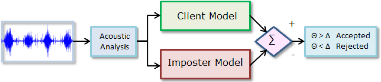
General Description of the Speaker Verification System workflow

ASV relies on modelling characteristics for each speaker in the system. Modelling is computed from training data and then a similitude is calculated between a model and the input signal and is used in the decision process.

6. Experiments and Data Sets

6.1 Commands Database in Mexican Spanish

In previous works [18], the database was composed of nine speech commands in Spanish: Arriba, Abajo, Derecha, Izquierda, Continúa, Inicia, Inicialízate, Para and Reinicia. The experiments were carried out obtaining MFCC vectors every 20ms over 30ms frames, while the present experiments used octile vectors in long-time and short-time. In the long-time configuration, a single vector is computed using the entire signal data, resulting in an 1 × q vector, where qq is the number of quantile coefficients. In the short-time configuration, a vector is computed every 300ms over 400ms frames, resulting in an n × q vector, where nn is the number of frames. In the MFCC experiments, a preprocessing stage was applied, while octile vectors were obtained as explained in Section 3. For experimental purposes, six speech commands were selected and tested applying octile vectors, with 52 recordings each.

6.2 XM2VTS Database

The experimental database is based on the XM2VTS ¹ database, which is multimodal, and has been used by the COST275 action partners (biometry over IP). XM2VTS comprises 295 different Speaker recording sets from Surrey University ² subjects, who were separated into four sessions, elapsed from one another by approximately a month per Speaker [25, 26]. The original audio files were recorded in three different phrases (each one recorded twice) and stored as WAV PCM files (sampled at 32 kHz, 16-bit, mono). Bearing in mind a possible future transmission over IP [16] and the parameters of our experiments, the Database was sub-sampled to 8 kHz. From now on, we will refer to this new database (the one used here) as XM2VTS8K.

6.3 Training and Testing Partitions

An already defined protocol for XM2VTS8K was adopted, known as the Lausanne protocol (Configuration II) [14, 26]. The XM2VTS8K database was split into three partitions: a training set (67%=199 Clients), an evaluation Set (8%=25 Impostors), and a test set (23%=70 Impostors). The training set is used to build the client model, while the evaluation set is used to compute the decision thresholds interval. The test set is used to compute the final system's efficiency. Sessions were only taken into account in the client partition.

Table 1.

Configuration for the XM2VTS8K Database Partitions (Lausanne Protocol)

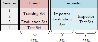
The training of the client model is performed using Sessions 1 and 2 from the client partition. The client test accesses are obtained using Session 4. The third client session and the impostor evaluation set were used to compute the thresholds interval.

6.4 Experimental Protocol using Octiles from the XM2VTS8K Database

At the beginning of the experimental protocol, an automated review of the database was performed to find which speaker folders existed and if they contained the expected 24 recordings. This examination criterion reduced the number to only 134 speaker folders. Two separated experiments were carried out with two speaker sets each: the first one with 134 speakers and the second one with 40. In both cases, 67% were used for the client model computation, 8% for evaluation purposes and the remaining 23% used as the impostor test set. This configuration is shown in Table 2.

Table 2.

Numbers of speaker corresponding to each partition

	XM2VTS8K Partitions	Client (67%)	Impostor Evaluation (8%)	Impostor Test (23%)
Speaker Qty.	134	90	11	33
	40	27	4	9

The fourth session of the client partition and the impostor test set were used to obtain the efficiency values. A priori, it was decided to compute the impostor model by using the whole database (i.e., 134 or 40 depending on the case).

This Background Model is computed with the purpose of representing speakers in general (referred to as UBM, Universal Background Model) [27]. If all speaker models were generated independently, some distributions of the mixture will probably not be trained or heavily under-trained. A posteriori, better results were looked for, so it was decided to carry out other experiments in which the impostor model would be computed with the impostor evaluation and impostor test partitions.

Once the client and the impostor models were computed, the evaluation sets were used only to determine the thresholds interval. After the thresholds interval was obtained, the maximum and minimum score values were used to determine a set of values, ranging from Δmin to Δmax, distributed in 101 levels (by a 0.01 step) in our case. Once the range is available, the test stage is carried out using the client and impostor test sets for each level, as shown in Figure 3. In this stage, the goal is to classify the audio files either as clients or impostors, which returns the quantity of false acceptations and false rejections. These quantities will be expressed as percentages, i.e., FAR and FRR values, respectively. Once the test stage is complete, the FAR and FRR curves' intersection is localized to obtain the EER.

The experiments were carried out in long-time and short-time. Long-time computation returns an 1 × 7 octile matrix for each recording, while short-time returns an 1 × 7 octile matrix for each recording, where n depends on the audio file time length, n

7. Results and discussion

The octile vectors were obtained from wav files in both short-time and long-time separately. They were calculated from the signal's frequency-amplitude spectrum, as shown in Table 3 and Figure 4.

Figure 4.

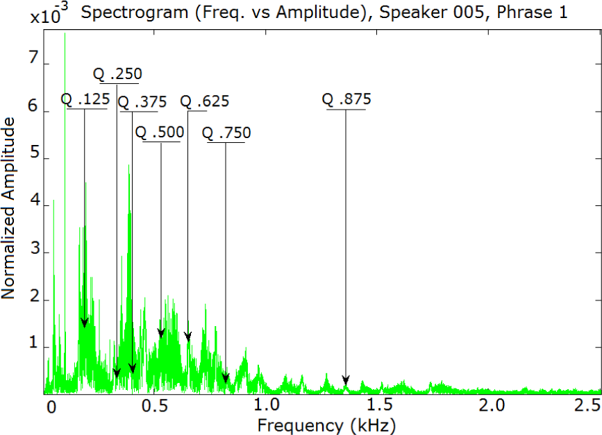
Frequency/Amplitude Spectrogram of Signal 005_1_1 and its octiles in long-time

Table 3.

Octile Vector from Speaker #005, Session 1, Phrase 1

Component:	Q.125	Q.250	Q.375	Q.500	Q.625	Q.750	Q.875
Frequency:	192 Hz	362 Hz	438 Hz	583 Hz	735 Hz	911 Hz	1294 Hz

Other experiments were carried out to analyse recognition improvements. For each speaker in the sets and their correspondent files, the silence segments were trimmed out (removed) manually. However, silence-removal did not show apparent recognition improvements.

Other spectral-based experiments were carried out in the hope of recognition improvements. These included anti-aliased FIR filters of the 200th order and the VAD algorithm (Voice Activity detection).

By means of an algorithmic and visual analysis of the recordings, FFT application, visual (at bare eye) spectrogram analysis and ear analysis for the 294 speakers (24 files each) issues in the recordings were noted. These included background noise and/or voices, device tones (beeps), mechanical noises (probably due to microphone manipulation), false speech starts and extended silences before and/or after speech. After all the recordings were analysed by ear, a set of 134 speakers was selected based on the recording quality. Additionally, a second set was selected from this last one, which consists of 40 speakers whose recognition efficiency was even better.

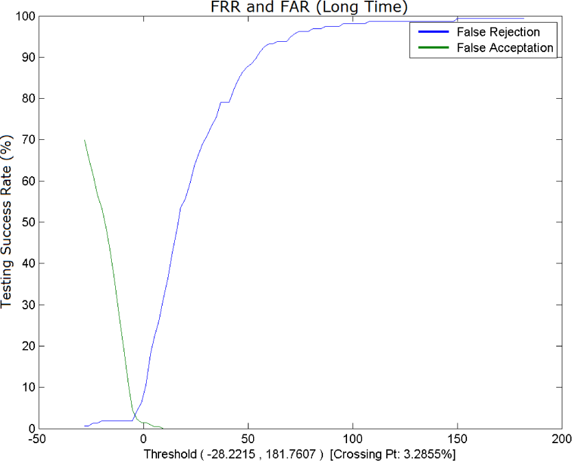
7.1 FRR (False Rejection Rate) and FAR (False Acceptation Rate)

After recording selection, the experiments were carried out by using all the speakers from each set to compute the impostor model: 134 or 40, depending on the case. The partitions (client, impostor-test and impostor-evaluation) were also made for each speaker set. However, the impostor model was computed in two ways: the first one was computed by using all the speaker sets and the second one was computed by using only the impostor partition. The results of the experiments can be seen in Table 4 and Table 5.

Table 4.

Obtained EER by using the whole speaker set to compute the impostor model

Gaussian Density	134 Speakers		40 Speakers
	Long T	Short T	Long T	Short T
1	41.78	53.23	36.53	60.28
2	44.13	51.89	35.89	56.81
3	45.20	52.97	33.93	57.62
4	42.31	52.66	33.59	49.89
5	44.11	53.27	34.31	48.82
6	42.68	NCP	35.64	53.94

Table 5.

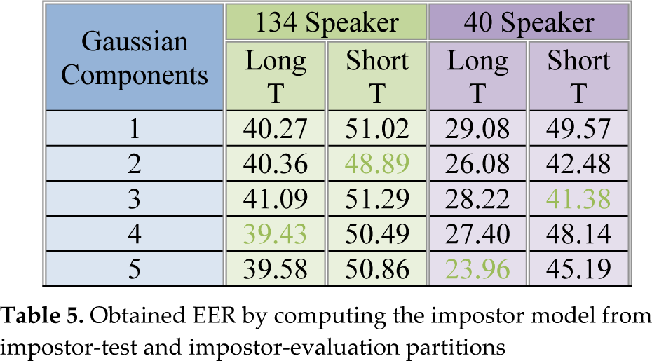
Obtained EER by computing the impostor model from impostor-test and impostor-evaluation partitions

Gaussian Components	134 Speaker		40 Speaker
	Long T	Short T	Long T	Short T
1	40.27	51.02	29.08	49.57
2	40.36	48.89	26.08	42.48
3	41.09	51.29	28.22	41.38
4	39.43	50.49	27.40	48.14
5	39.58	50.86	23.96	45.19

First, Table 4. shows the results for the experiment where the impostor model was computed from the entire speaker set.

The recognition improvement shown in the case of 40 speakers (long-time) can be explained by the fact that the relation between the total classes to recognize and total data is lower than in the case of 134 Speakers.

Subsequently, the experiments were done in a different configuration: this time the impostor model was built by using only the impostor-test and impostor-evaluation partitions, as shown in Table 5.

As seen in Figures 5 to 8, it is evident that a good selection of the data partitions (cohort or world model) largely improves the results. In order to improve the results, it is necessary to analyse the used method to build the models (Impostor, particularly).

Figure 5.

EER=41.78 for 134 Speakers. Impostor Model was built with all 134 Speakers.

Figure 6.

EER=33.59 for 40 Speakers. Impostor Model built with all 40 Speakers.

Figure 7.

EER=39.43 for 134 Speakers. Impostor model built with Impostor-Test and Impostor-Evaluation.

Figure 8.

EER=23.96 for 40 Speakers. Impostor Model built with Impostor-Test and Impostor-Evaluation.

Finally, an additional experiment with the 40 speaker set was carried out, applying quantiles in Mel-scale (13 coefficients) and MFCC in the same experimental environment for comparison. Here, the Impostor model was computed from the impostor-test partition, as shown in Table 6. It is important to mention that octile vectors were applied in previous work [28], regarding lung sounds verification, which obtained excellent results; lungs sounds are similar to noisy signals, so octile vectors could be useful for this kind of signals, but this remains another future work.

Table 6.

Obtained EER (in percentage) for the 40 speaker set. Impostor model computed from the set's impostor-test and impostor-evaluation partitions.

Gaussian Components	40 Speakers, QMel (logFTT)		40 Speakers, Classic MFCC
	Long T	Short T	Long T	Short T
1	28.5784	28.3586	15.65	29.79
2	23.6590	33.2812	13.79	28.81
3	22.8965	30.2668	15.81	30.68
4	24.3124	34.2536	13.14	25.32
5	19.9643	28.3333	11.25	26.98
6	18.8087	34.7095	7.40	27.77
10	15.5193	27.9835	8.78	22.89
20	10.5232	25.6543	7.22	20.59
30	9.3034	19.5710	4.29	16.42
64	4.5875	18.2411	2.63	8.33
128	2.4691	11.0306	1.46	4.62
130	1.8519	11.2140	0.56	3.53
132	1.5873	13.1944	1.23	4.29
150	0.5698	10.7666	15.65	29.79

In the first experiments (Table 4) the number of Gaussian densities needed to be increased in order to invert the recognition efficiency tendency, while in the last experiment the efficiency kept improving until 130 Gaussian densities. These last results (3.28 EER particularly) are very encouraging and support our approach.

Figure 9.

EER=3.28 for 40 Speakers. Impostor Model was built with Impostor-Test and Impostor-Evaluation partitions.

7.2 Octile Vectors in Command Recognition

In Section 2, MFCC vectors were presented with experiments in command recognition, but the results suggested producing another alternative in order to improve the recognition system. Such an alternative should be computationally less expensive. Therefore, we carried out command recognition by applying octile vectors and the results are shown in Table 7 and Table 8.

Table 7.

Long-time Command Recognition (1 Vector per Recording)

	Number of Gaussian Densities
	1	10	28
Overall Command Recognition	55.8%	82.4%	96.5%

Table 8.

Short-time Command Recognition (1 Vector every 300ms in 400ms frames)

	Number of Gaussian Densities
	10	20	30	35	40	50
Overall Command Recognition	86.21%	92.62%	97.11%	98.71%	98.71%	99.35%

In Table 7, the results of three long-time experiments are presented: one, ten and 28 Gaussian densities. The accuracy recognition was averaged for the six commands applying octile vectors. Table 8 shows the results for six short-time experiments: 10, 20, 30, 35, 40 and 50 Gaussian densities, also averaging the results for the six commands. From Table 7 and Table 8, it is possible to see that the results are acceptable, even in long-time, compared to the results obtained from the computationally more expensive MFCC vectors.

The MFCC is a successful front-end technique in speech recognition, but apparently, quantile vectors obtain more representative frequency values and maybe a better trade-off between energy and frequency characteristics.

7.3 A Comparison between Octile and MFCC Acoustic Vectors

In order to explore the benefits of using octile vectors, the following facts have arisen along the verification experiments:

In general, our SVS system (using an Intel i5 microprocessor @ 2.5 GHz, Laptop), in long- and short-time requires, on average, 35% less time to compute octiles in comparison to MFCC.

The obtained EER results were 0.5698% using octiles with 150 densities and 0.56% for MFCC.

Regarding the complete verification process, from vectorization to EER, computation times are similar for both cases. This is more noticeable as the number of mixtures increases.

In regards to model storage, as computed in Table 6, the storage space between the Mel-scaled quantile and MFCC vectors is equal, since the values were computed in a fixed-point algorithm.

Previous work in speaker verification using the XM2VTS database [16, 19] reported 0.25% EER. The system used 32 LFCC coefficient vectors, models of 128 densities and the ELISA toolkit (a modern version of ALIZE [29], developed by the Informatics Lab at Avignon University). In comparison to our octile-based models, the reported LFCC vectors are inconvenient in autonomous and energy-limited systems considering their use of 18.52 times more storage space.

Additionally, our SVS system is still improving. The system could be optimized at an algorithmic and computational level; consequently, we expect to attain better computation times and/or overall efficiency.

8. Conclusions and future Work

In this paper a novel acoustic vector approach was presented, which was inspired by breathing flow intensity experiments and also considering the time interval stationarity of such events.

Two acoustical vector lengths were evaluated: long-time and short-time. Both methods showed encouraging results, especially using quantile vectors in long-time analysis, which is different from most papers in the literature. Long-time analysis is less expensive than short-time analysis; in Table 6, most of the best verification results were obtained in long-time analysis. GMM model computation with a higher number of Gaussian curves (up to 150) gave us the best results in terms of EER (0.5698%).

The quantile acoustic vectors have the advantage of relating signal energy with its more relevant frequency values. In fact, our presented method offers a good tradeoff between computation times, characteristics vector complexity and overall obtained efficiency. Curiously, the long-time alternative (in which computation is relatively less expensive) presented the best results in speaker verification.

In an autonomous systems context, the command recognition achieved very good results: 96.5% overall accuracy recognition in long-time with 28 Gaussian densities and 99.35% overall accuracy in short-time configuration. Consequently, quantile vectors have good expectations in the autonomous systems context, due to a less expensive front-end.

The experiments are encouraging, given the relative simplicity of the octiles vectors in comparison to those previously mentioned, such as MFCC. They were obtained from a non-preprocessed audio signal, which leaves us the possibility to improve our results in the future, by including some kind of preprocessing.

Our approach of octiles vectors was motivated by the inquiry into which frequency values were most relevant in an acoustic vector and how their energy is related to the signal formants.

In the future, we will examine some of the system's stages and experiment with VAD (Voice Activity Detection) and CMS preprocessing being more exhaustive in the analysis of representative frequency values to improve recognition efficiency.