
Abstract
Abstract Technological advances combined with the demand of cost efficiency and environmental considerations has led farmers to review their practices towards the adoption of new managerial approaches, including enhanced automation. The application of field robots is one of the most promising advances among automation technologies. Since the primary goal of an agricultural vehicle is the complete coverage of the cropped area within a field, an essential prerequisite is the capability of the mobile unit to cover the whole field area autonomously. In this paper, the main objective is to develop an approach for coverage planning for agricultural operations involving the presence of obstacle areas within the field area. The developed approach involves a series of stages including the generation of field-work tracks in the field polygon, the clustering of the tracks into blocks taking into account the in-field obstacle areas, the headland paths generation for the field and each obstacle area, the implementation of a genetic algorithm to optimize the sequence that the field robot vehicle will follow to visit the blocks and an algorithmic generation of the task sequences derived from the farmer practices. This approach has proven that it is possible to capture the practices of farmers and embed these practices in an algorithmic description providing a complete field area coverage plan in a form prepared for execution by the navigation system of a field robot.
1. Introduction
Technological advances combined with the demand for cost efficiency and environmental considerations require farmers to reconsider their practices and adopt new managerial approaches including enhanced automation [1]. The application of new technologies, which is able to maximize the operational efficiency of the system in a way that optimizes the use of scarce resources and minimizes the environmental impact, is needed [2]. The application of field robots is one of the most promising applications of these automation technologies.
Emerging field robots are required to operate with minimum human intervention but also in an efficient and safe way. Since the primary goal of an agricultural vehicle is the complete coverage of the cropped area of a field, an essential prerequisite is the capability of the mobile unit to cover the field area parts autonomously. An automated machine needs a planned path directing the execution of the operation. The boundaries of a field and its obstacle areas are usually fixed from year to year, providing a predetermined environment where the resultant paths could be deterministic and known in advance.
Coverage path planning for field operations is a special case of the general problem of path planning for outdoor environments (e.g., [3]). Due to the semi-structural environment, both on-line planning based on sensor fusion (e.g., [4–5]) and off-line planning can be applied. Regarding the off-line planning for field area coverage, a number of approaches have been presented. The first step for complete off-line planning is the solution of the problem of the geometrical representation of the field as an operational environment. In [6] a field geometrical representation algorithm is presented, which can generate straight and curved tracks and treats a field as a single region or divides it into sub-regions and generates field work tracks parallel to the longest edge of the field/sub-region. This method has also been applied in non-agricultural domains such as planning operations including the planning of grass cutting operations in football stadiums [7]. Pursued methods have also taken into consideration biodiversity issues, as for example in [8]. Regarding the specific coverage planning procedure pertained to such generated operational environments, a number of methods have been introduced. In [9] and [10] the algorithmically-computed optimal fieldwork patterns, the B-patterns, are presented, which provide optimal fieldwork track sequencing according to the criterion of minimizing the non-working travelled distance of an agricultural vehicle. In [11] a genetic algorithm based approach for the simultaneous selection of the driving line direction and sequence of tracks that minimizes operational time and overlapped areas was derived. In the case of field operations in rolling terrains the terrain characteristics (i.e., for example elevation) have a significant influence on the design and optimization of the coverage path planning. A route planning method for agricultural vehicles carrying time-dependent loads with the objective of reducing the risk of soil compaction was presented in [12]. In [13] a 3D geometrical field representation combined with a simulation tool for field operations under capacity constraints is presented. The developed tool can represent a field more accurately in a 3D environment using the digital elevation model (DEM) of the field's area and therefore can be used for more realistic optimization of various field operations and for more accurate robot navigation.
There are some mobile-robot applications that require the complete coverage of an unstructured environment. Examples are humanitarian de-mining, floor-cleaning tasks and tasks in agriculture. A complete-coverage algorithm is then used, a path-planning technique that allows the robot to pass over all points in the environment in a systematic way, avoiding unknown obstacles. Different coverage algorithms exist, but they fail to work in unstructured environments. In some applications, such as in agriculture, the task becomes more complex since an autonomous vehicle or a robot has to drive in rows in order to minimize crop damage and to simplify the cooperation between a set of autonomous vehicles in carrying out a single task [11–13]. A variety of coverage algorithms exist [14–21], but the most powerful ones are those that rely on finding the critical points of a function to guarantee the completeness of the method [16–20]. Liu and Palmer [14] developed an approach based on graph theory for formulating efficient courses around an obstacle. Obstacles that are less than four implement widths should be circumvented with each pass. Larger obstacles should have a headland with each side of the obstacle being processed separately. This approach works well for simple obstacle shapes, however it requires, under some circumstances, human intervention for making hard decisions. Lumelsky et al. [15] presented a dynamic path planning approach based on a vision system where the task is accomplished by walking from one obstacle to the other in order to build a terrain map. Zelinsky et al. [16] presented an approach for generating a path from a start location to a goal location, while minimising one or more parameters such as length of path, energy consumption or journey time where a robot sweeps all the areas of the free space in a systematic and efficient manner. This approach can be used by autonomous vacuum cleaners, lawn mowers, security robots and land mine detectors but cannot be used in applications where crops are planted in rows. In [17–19], an approach based on the formulation of cellular decompositions of an unknown space using critical points of Morse functions is presented. The critical point formulation forms simple cells that can be covered by performing simple motions, such as back and forth. Garcia and Gonzalez de Santos [20] described a method for complete track coverage of unstructured environments incorporating obstacle avoidance. The method was based on exact cellular decomposition of a field. With this decomposition it was possible to divide a field with obstacles into subfields (cells) containing no obstacles. The drawback of this approach is the unvisited subfields, which can cause an economical loss to farmers. In [21] a grid representation for the field and a genetic algorithm (GA) were used to find the optimal path travelling through all the grids and hence covering the entire field area. Nevertheless, the method does not provide paths that are feasible for all field operations, e.g., in the case of row crops.
In this paper, the main objective is to develop an approach for coverage planning for agricultural operations involving the presence of obstacle areas within the field area. The aim of the approach is to capture the prevailing practices of farmers, and if possible to optimize such practices and provide a complete field area coverage plan that is executable by the navigation system of an agricultural field robot. The developed approach does not require any human intervention and can deal with any field regardless of the complexity of its shape and the number of the shape complexity of its obstacles.
2. Methodological approach
2.1 Geometrical representation
The developed approach includes three stages. In the first stage, the field polygon is filled with field tracks parallel to a user-defined angle (i.e., driving angle). The driving angle can also be optimized in a manner that reduces, for example, operational time, soil compaction or emitted CO2 as a result of the vehicle's activities, etc. (see [11–13]). In the second stage, the generated tracks are arranged and clustered into sub-fields (referred to as blocks) taking into account the in-field obstacles. In the third stage, headland paths are generated at the upper and lower sides of the tracks in each block. Each stage will be explained in detail in the following sections.
2.1.1 First stage: track generation
In this stage, the field boundary and the boundaries of the in-field obstacle areas are firstly inputted using a user-provided source shape/text file. The minimum bounding box (MBB) of the field boundary is then generated and filled with straight lines parallel to a user-defined driving angle, θ, spaced by a distance equal to a user-defined operating width, w. The driving angle is defined as the angle between the driving direction and a horizontal reference x-axis (e.g., the UTM Easting axis). The intersection between each track line and the field outer boundary or the boundaries of the obstacle areas are then obtained. The parts of the tracks contained within the field boundary are maintained, while the remaining parts are eliminated. More details of this process can be found in [6]. As an example, the blue line of the field shown in Fig. 1a, represents the field outer boundary, while the red line represents the boundary of an obstacle area. Generated field tracks for two selected driving angles are shown in Fig. 1b and Fig. 1c.

The outer boundary of a field (blue polygon) and the boundary of an in-field obstacle (red polygon) [+56° 29′ 14.01“, +9° 32′ 33.33”] (a) examples of generated field tracks for two selected driving angles (b) θ = 45° (c) θ = 90°
2.1.2 Second stage: clustering of field tracks
A track generated in the first stage, is defined as a line segment, which intersects the field outer boundary in the form of two end points. Let T0 = (1,2,3, …} denote the set of these initial tracks. If a track intersects with an in-field obstacle area, then it can be divided into two independent tracks, each track having two end points with one end point located on the field outer boundary and the other end point located on the boundary of the intersecting obstacle boundary.
In the general case, if a track i ∈ T0 has ni intersections, then it crosses ni/2 − 1 obstacle area parts and can be subdivided into mi = ni / 2 segments, which make up the new tracks. For n = 2, the track intersects no obstacles and therefore it is undividable. The total number of the new generated tracks can be obtained as
The next step involves clustering of the generated tracks into blocks. The clustering process starts by checking the possible subdivision of a specific sequenced track. If the current track can be divided into mi tracks, then mi empty blocks are created and the generated tracks are allocated to these blocks in sequence. If the next track in the sequence is expressed as mi+1 = mi, the new mi+1 tracks are saved in the current mi blocks. On the other hand, if mi+1 ≠ mi then mi + 1 new empty blocks are created then the new generated tracks are saved in the new blocks in sequence. A pseudo-code of the clustering process is listed in Table 1. It should be noted that the number of the generated blocks depends on the selected driving angle and consequently on the driving direction. For example, Fig. 2 presents a virtual field with two obstacles and different number of resulting blocks for two different driving directions.
The pseudo-code of the track clustering process


The effect of driving direction on the number of field blocks for a field with two obstacles
2.1.3 Third stage: headland polygons generation
In a field operation, headlands are created by the sequential passes that the agricultural machine has to perform peripherally to the main field area and around each obstacle area (Fig. 2). A headland area consists of a sequence of internal (or external in the case of an obstacle area) boundaries corresponding to headland passes. The width of the headland area results from the multiplication of the effective operating width of the machine by the number of the peripheral passes. Let h denote the number of the headland passes. The distance between the first headland pass and the field boundary is half of the implement width, w / 2, while the distance between subsequent headland passes equals an implement width w, where w denotes the (effective) operating width of the operating implement. A headland path is obtained by acquiring the intersection points between segments of lines parallel to the segments of lines of the previous headland pass at distance d to the interior of the field area or the exterior area in the case of an obstacle. The distance d for the first headland pass is set to w / 2, while for the rest of the passes it is set to w. An additional (virtual) headland pass is generated at distance w / 2 from the last headland pass to be used as the internal boundary of the main field area, as is shown in Fig. 3.

Creation of headland passes polygons: point a is the intersection of the track with the field outer boundary (black line), point b is at half operating width from the field outer boundary, point c is at full operating width from previous headland pass, and point d at half operating width from the last headland pass
2.2 Block sequence optimization
For a field robot to carry out an agricultural operation without crossing any field obstacles it should cover each block of tracks one at a time and therefore it is required to find the optimal covering order of the generated blocks. This problem can be formulated as an optimization problem where the decision variable is the order of blocks and the objective function to be minimized is the total connection distance between blocks.
Let B = {1, 2, 3, …} denote the set of generated blocks and let xij,i, j ∈ B / i ≠ j denote the decision variables of the problem where xij = 1 if the vehicle after block i transfers to block j and xij = 0 otherwise. The objective function of the problem is

Entrance points are arranged in clock-wise direction (a) a block with odd number of tracks (b) a block with even number of tracks
The exit point of a block is a function of the entrance point as derived by the configuration of the field tracks. Let f(·):{1, …, 4}→{1, …, 4} express the function that a specific entrance connection point results in a specific connection point. In the case of an odd number of field tracks in a block f(1) = 3, f(2) = 4, f(3) = 1 and f(4) = 2, while in the case of even number of tracks in the block then f(1) = 4, f(2) = 3, f(3) = 2 and f(4) = 1.
2.2.1 Small-scale problems (SSP)
In this context, SSP are defined as a problem, which has a number of blocks |B| < 4. For four blocks, there are up to 24 (i.e.,|B|!) candidate solutions with repetitions or 12 candidate solutions without repetitions. In this type of problem, all possible sequences can be easily obtained using random permutation within B. A real-valued genetic algorithm (RGA) is applied to find the optimum entrance points for each respective block in each sequence of blocks (i.e., candidate solutions). A chromosome constitutes of |B| genes where each gene has an integer value in the range of [1, 4], as is shown in Fig. 5a. The connection distance for each solution is saved and the one with minimum connection distance is returned. The advantage of this type of problems is that a global optimum solution is guaranteed, however, it is time consuming and not practical for problems of more than four blocks.
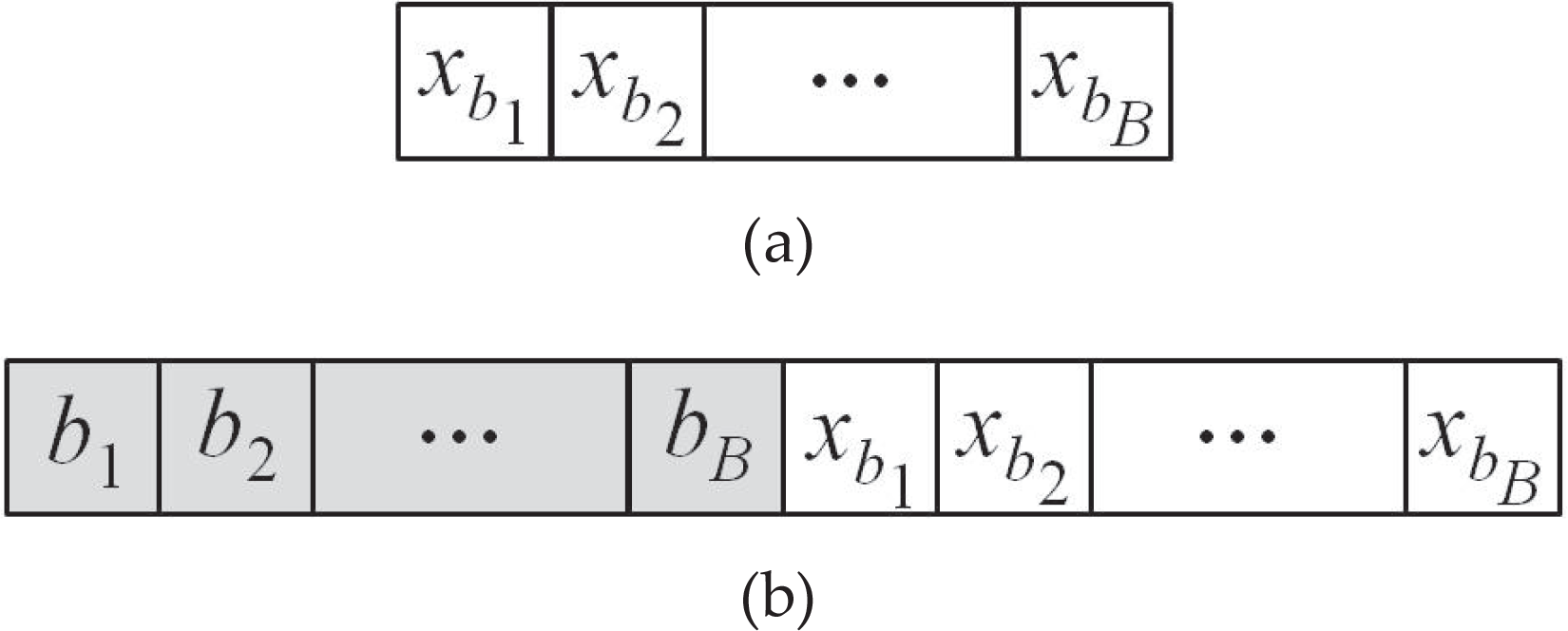
Chromosome structure (a) coding of entrance points of blocks optimizing entrance points of field blocks (b) coding of block sequence in the first half and entrance points in the second half of the chromosome
2.2.1 Large-scale problems (LSP)
For more than four blocks, an RGA can be used to find both the optimal sequence of blocks and, at the same time, the optimum entrance point of each respective block. The sequence of blocks is encoded in permutation and constitutes the first half of the chromosome while the entrance points of the respective blocks constitute the second half of the chromosome. The chromosome structure for solving this type of problem is shown in Fig. 5b. The advantage of these types of problems is their quick convergence but at the cost of having an optimized solution where there is no guarantee that the obtained solution is the global optimum.
2.2.3 Real-valued genetic algorithm (RGA)
The input to the block-sequencing problem is two sequenced set of integers, where the first set of integers represents different blocks together with the order representing the time at which a block must be visited and a second set of integers where each integer represents a block entrance point. The output of the problem is the connection distance between blocks measured using Euclidean distance over 2D space. The decision variables are represented by the sequences of blocks, which are permutationally encoded, and entrance points, which are real-valued and encoded. Real-valued encoding not only reduces computational efforts but also speeds up convergence. The performance of the GA depends on the crossover and the mutation operators of the GA [22]. The type and the implementation of operators depend on the encoding and also on the underlying problem. In real-valued encoding, every chromosome is a string of values. Values can be anything connected to the underlying problem, from numbers, real numbers or charts to complicated objects. In real-valued encoding, crossover operators used in binary encoding are applicable where parts of the strings from two parent chromosomes are swapped in order to produce two new off-spring [23]. Mutation is carried out by adding or subtracting a small value to a selected gene value. In the case of integer values, this value is rounded to the nearest integer after the addition or subtraction.
In permutation encoding, every chromosome is a string or a sequence of integers, where each integer represents a different block and the order represents the time at which a block is visited. Permutation encoding can be used in ordering problems, such as the travelling salesman problem (TSP) or task ordering problems. In this case, each block has to be visited once and no blocks can be discarded. Also, a scheme analogous to simple crossover is required, but one which preserves solution viability while allowing the exchange of ordering information. One such scheme, among others, is partially matched crossover (PMX). In this scheme, a crossing region is chosen by selecting two crossing sites at random. Crossover is performed in the centre region. Replicated alleles in the crossing region are replaced by cross-referencing with the parent of the alternate chromosome [24]. Mutation is often used in GAs as a way of adding random variation to the evolving population, preventing a total loss of diversity. To avoid a resulting non-viable block order, inversion mutation is used, in which a randomized exchange of alleles in a randomized chosen chromosome is applied. This can be accomplished by applying a given (usually small) probability, much like mutation.
2.3 Generation of the final path
The sequence of the visited blocks and the sequence of traversing the tracks within each block cannot provide by themselves an executable and complete coverage of the field area. The reason for this is that in field operations, as mentioned earlier, auxiliary paths in terms of headland passes are needed in order to complete the operation. The execution time for these paths, i.e., prior or after finishing the main area coverage, depends on the type of operation. In the case of a material input operation (e.g., seeding), the headland passes are executed after the completion of the operation in the main area. In the case of output material operations (e.g., harvesting), the headland passes are executed prior to the operation in the main area.
In order to produce a complete coverage plan that includes both the traversal sequence between the tracks as well as the headland passes, two algorithms were developed, one for input material flow operations and one for output material flow operations, incorporating the task execution practices that have to be followed in agricultural operations. Fig. 6 and Fig. 7 represent the flow diagrams depicting the two algorithms representing input material flow operations (for example, the seeding operation) and material output operations (for example, the harvesting operation), respectively.
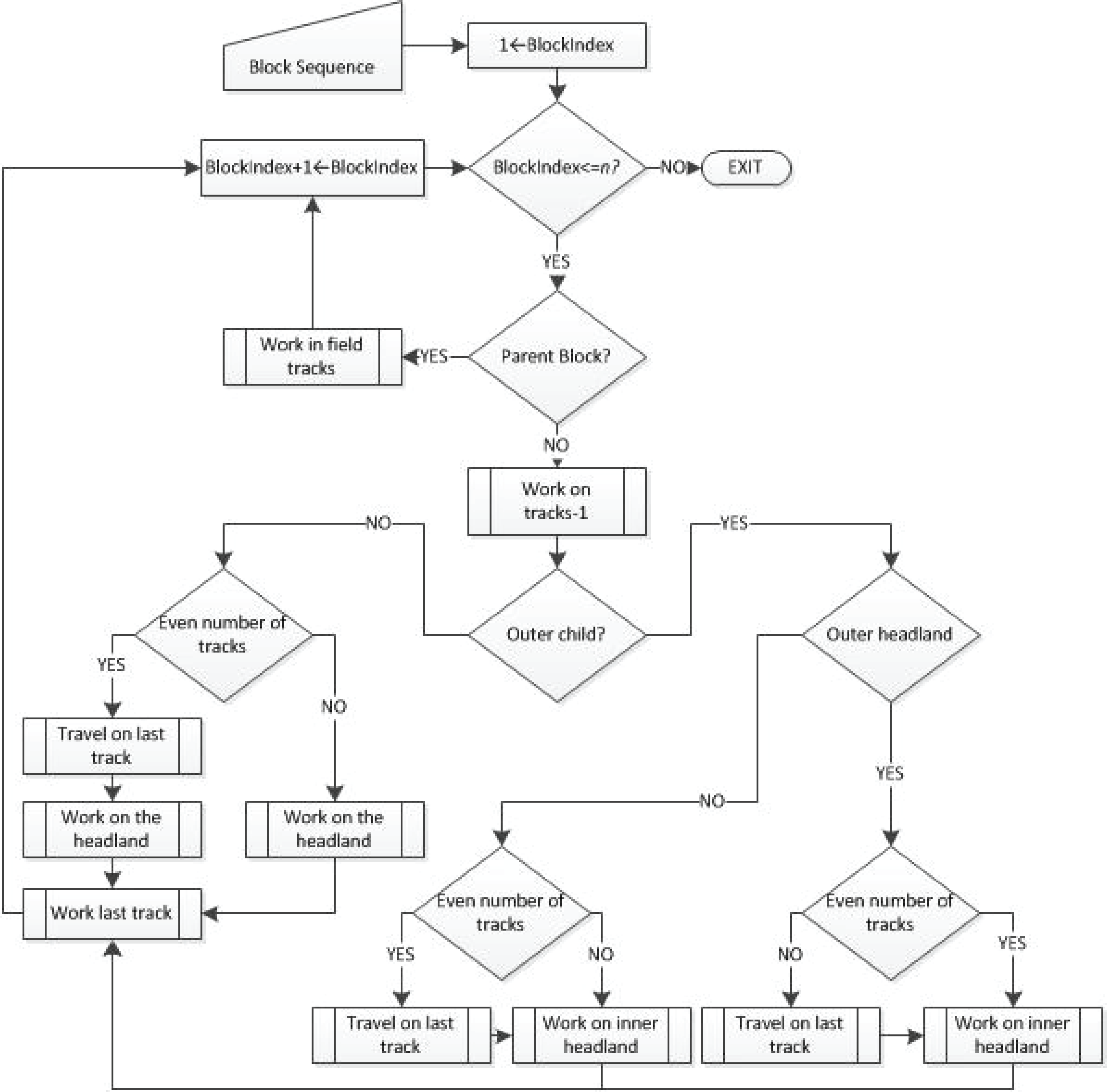
The flow diagram for the generation of the final path in the case of input material flow operations

The flow diagram for the generation of the final path in the case of output material flow operations
3. Results
3.1 SSP example
The first demonstration field [+54° 57′ 8.28″ E, +9° 46′ 49.31”N], shown in Fig. 8a, has an area of 5.54ha or 55375.38m2 and has one obstacle area. The coverage planning is generated for a driving angle of 4.5° and an operating width of 9m and two headland passes. The developed coverage planning approach is applied to this field and the field tracks are clustered into four blocks, as is shown in Fig. 8b. The computational time for this operation was 0.18 seconds as an average of ten running times on an average computer. The field has four blocks so it could be classified as an SSP and therefore the general GA was used to find the optimum entrance point for all possible permutations of block sequences (i.e., for 4! = 24 block sequences). The default sequences of tracks in each block are given in Table 2.
Indices of after division tracks in each block


Test field 1 (a) A field of a single obstacle area (i.e., SSP type) (b) the block generation for a selected driving angle of 45°, a working width of 9m and two passes in the headland area
The sequence of the blocks and the corresponding entrance and exit connection points are shown in Fig. 9. There are two optimal solutions, as is shown in Table 3. It is worth noting that the two solutions are identical but one is the reverse of the other. The two solutions are graphically shown in Fig. 9. The solution was obtained in 0.47 minutes (as an average of ten running times on an average computer) using an RGA of a population size of 100, 50 generations and 0.8 and 0.01 crossover and mutation probability, respectively.
Optimal block sequence

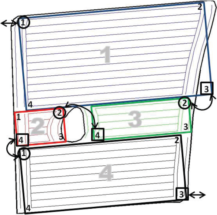
Illustration of the two equivalent optimum solutions of experimental field 1: circles and squares could be either entrance or exit points and vice versa
3.2 LSP example
The second experimental field [+56° 30′ 26.79“, +9° 36′ 54.35”], shown in Fig. 10a, has an area of 94.03ha (i.e., 940,309.60m2) and two in-field obstacle areas. An operating width of 18m and two headland passes were assumed, together with a driving angle of 84°. The field representation after clustering 67 tracks into 7 blocks is shown in Fig. 10b. The block generation was obtained in an average time of 0.28 seconds (average of ten running times on an average computer).

Test field 2 (a) A field with two obstacle areas (of LSP type) (b) The block generation for a selected driving angle of 84°, working width of 9m and two passes in the headland area
For seven blocks, there are 5040 different sequences of permutations. The RGA was used to find the best sequence of blocks. The solution was obtained in 14.41 minutes (as an average of ten running times on an average computer) and a minimum connection distance of 610.04m was achieved. The default sequence of tracks in each block is shown in Table 4, while the resultant optimized solution is shown in Table 5. In this problem, a mixed permutation and real-valued encoded GA of a population size of 100, a maximum generation number of 100, a crossover probability of 0.8 and a mutation probability of 0.01 were used. The solution is graphically shown in Fig. 11.
Indices of after division tracks in each block

Optimal block sequence

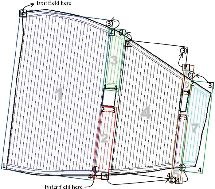
Illustration of the obtained optimized solutions of experimental field 2: circles and squares represent entrance and exit points to and from a block respectively
4. Conclusions
The developed approach for coverage planning for agricultural operations involving the presence of obstacle areas within the field area provides the necessary information required for aiding and supporting navigation of field robots in such complex fields. The performance of the optimization algorithms used to optimize the coverage planning requires relatively low computational times compared to an off-line planning system. This approach has proven that it is possible to capture the practices of farmers and embed these practices in an algorithmic description providing a complete field area coverage plan in a form prepared for execution by the navigation system of a field robot. Moreover, in the case of complex fields in terms of the number of obstacle areas, the approach can provide an optimized plan that enhances the farmer's practice.