Modelling,Specification and Robustness Issues for Robotic Manipulation Tasks

Abstract

In this paper, a system for modeling of service robot tasks is presented. Our work is motivated by the idea that a robotic task may be represented as a set of tractable modules each responsible for a certain part of the task. For general fetch-and-carry robotic applications, there will be varying demands for precision and degrees of freedom involved depending on complexity of the individual module. The particular research problem considered here is the development of a system that supports simple design of complex tasks from a set of basic primitives. The three system levels considered are: i) task graph generation which allows the user to easily design or model a task, ii) task graph execution which executes the task graph, and iii) at the lowest level, the specification and development of primitives required for general fetch-and-carry robotic applications. In terms of robustness, we believe that one way of increasing the robustness of the whole system is by increasing the robustness of individual modules. In particular, we consider a number of different parameters that effect the performance of a model-based tracking system. Parameters such as color channels, feature detection, validation gates, outliers rejection and feature selection are considered here and their affect to the overall system performance is discussed. Experimental evaluation shows how some of these parameters can successfully be evaluated (learned) on-line and consequently improve the performance of the system.

1. Introduction

Humans facilitate complex coordination between the eye and the hand during execution of everyday activities such as pointing, grasping, reaching, catching and various tool manipulation. Each of these activities or actions require attention to different attributes in the environment - while pointing requires only an approximate location of the object in the visual field, a reaching or grasping movement require more exact information about the object's pose. An extensive study of human visually guided grasps in (Hu et al, 1999) has shown that the human visuomotor system takes into account the three dimensional geometric features rather than the two dimensional projected image of the target objects to plan and control the required movements. In robotics, the use of visual feedback for coordination of a robotic arm motion is termed visual servoing, (Hutchinson et al, 1996). Compared to most of the current robotic visual servoing systems, which are image based and based on 2D feature tracking, the information used by humans is much more complex and permits humans to operate in large range of environments. To develop robust and safe robotic manipulation systems, we have to consider and solve problems such as autonomous navigation, obstacle avoidance, object recognition and grasping as well as design of a robot architecture that will support their coordination. In this paper, we consider just two of the above problems guided by the motivation that a key to solving robotic hand-eye tasks efficiently and robustly is to identify how precise control is needed at a particular time during task execution. Here, three levels may be considered:

Transport considers motion of the robot plat form/arm to the vicinity of the object.

Alignment of the hand with the object such that a grasp can be performed.

Grasping of the object which can be performed using tactile feedback or in a predefined open-loop manner.

In terms of visual feedback during the transport phase, coarse 2D information may be sufficient. However, for object manipulation and grasping it is usually required to accurately estimate the position and orientation (pose) of the object to, for example, allow the alignment of the robot arm with the object or to generate a feasible grasp and grasp the object. Consequently, it is obvious that for service robot applications, it is of inevitable importance to observe the complete robotic task considering varying levels of complexity for each step. As an example, assuming basic fetch-and-carry tasks, there will be varying demands for precision and degrees of freedom controlled at each step. The required level of precision should then be matched with appropriate sensory input. A system based on this idea is presented in the first part of the paper.

In terms of sensors, computational vision is frequently used to provide the necessary feedback for the control loop. Realistic environments (tables, shelfs) and natural objects (such as food packages, cups, etc.) offer us very little place for assumptions such as, for example, uniform color or simple texture attributes. A number of model-based pose tracking systems have been proposed in the literature (Armstrong & Zisserman, 1995), (Vincze et al, 1999), (Wunsch & Hirzinger, 1997), (Drummond & Cipolla, 2000), (Lowe, 1985). One common feature for all of them is the use of wireframe models and object features to estimate current pose/velocity of the object. Most of them deal with tracking of particular targets (e.g. cars), usually uniform in color with a moderately varying backgrounds.

Our paper provides an experimental appraisal of the parameter issue in a model based tracking system. The main objective is to present the different parameters that affect the performance of a model-based tracking system and integrate some of the ideas proposed in the above mentioned systems to achieve robustness in terms of tracking of textured objects in everyday environments.

Our system has successfully been used to: i) estimate the pose of an object to be grasped, and ii) track the pose of an object for cases of moving camera/moving robot tasks. The system is model based and uses a number of ideas proposed in other similar systems and integrates these to successfully cope with partial occlusions of the object and to maintain tracking of the object even in the case of significant rotational motion and background clutter. The ability to cope with occlusions and changes in the appearance of the object are two of the capabilities required for the design of a robust tracking and visual servoing system.

The paper is organized as follows. In Section 2, the basic design of the system is presented. In Section 3, a model based tracking system is presented followed by the parameter issue in Section 4. In Section 5, a detailed experimental evaluation is performed. Finally, in Section 6 a short summary is given and avenues for future research are outlined.

2. The system

In the development of our system, the following issues were considered:

i)

The system has to be modular - complex tasks should be defined using a set of basic control primitives. This allows to model a variety of tasks using the existing architecture.

ii)

The system should be flexible to allow the users to easily change the existing model for the task they want to perform.

iii)

The system should be scalable so that that the system structure executes both simple and complex tasks with same efficiency.

iv)

And finally, the system should have a theoretical foundation that allows for synthesis and verification.

The current system is composed of three levels shown in Fig. 1:

Fig. 1.

System architecture.

• i)

  Task graph modeling and generation allows the user to design and generate a graph for the task he/she wants to perform.

• ii)

  Task graph execution - given the task graph, the system automatically initiates all the basic processes required to execute the task.

• iii)

  A set of basic primitives is implemented and used during the execution of the first two levels. These primitives are the ones commonly required for service robot tasks. Our previous work provides a detailed presentation of all the primitives currently available in the system, (Kragic & Christensen, 2003).

2.1. Basic Primitives

The instructions to the low-level motion controller of the robot are passed from the basic primitives. The primitives have a common interface with functions such as Start(), Run() and Stop(). The core functions are defined in a base class, so if the user wants to design a new module, all the basic functionality is inherited from the base class and only the module specific parts have to be implemented. Our assumption is that tasks consist of discrete, serial, quasi-static steps, each with a clearly defined outcome. Hence, models for such procedures can be defined by relatively simple graphs, (Kragic & Christensen, 2002).

2.2. Task Specification

Our system has originally been designed for Human Machine Collaborative Systems for surgical interventions, (Kragic & Hager, 2003). Here, we have assumed that the interventions can be modeled by a set of events, basis vectors and a procedure with a sequence of states. Events represent links or triggers between the states and are either sensory based (e.g. contact detected) or induced by the user (e.g. button pressed or predefined pose). Basis vectors span the task space of the robot. Using different types of operators on the basis vectors, we can easily define subspaces for preferred robot motion. States are represented by a set of transitions and constraints. Transitions are pairs (event, newState), i.e. for each event there is a newState defined.

Given a set of basic primitives representing individual states these can be combined to design complex tasks. Here, the important feature of the system is therefore the ability to impose some basic requirements on the design of a task. For this reason, we have chosen to use the XML Schema Definition Language (XSD), (www.xml.org) based representation for a general class of tasks as follows:

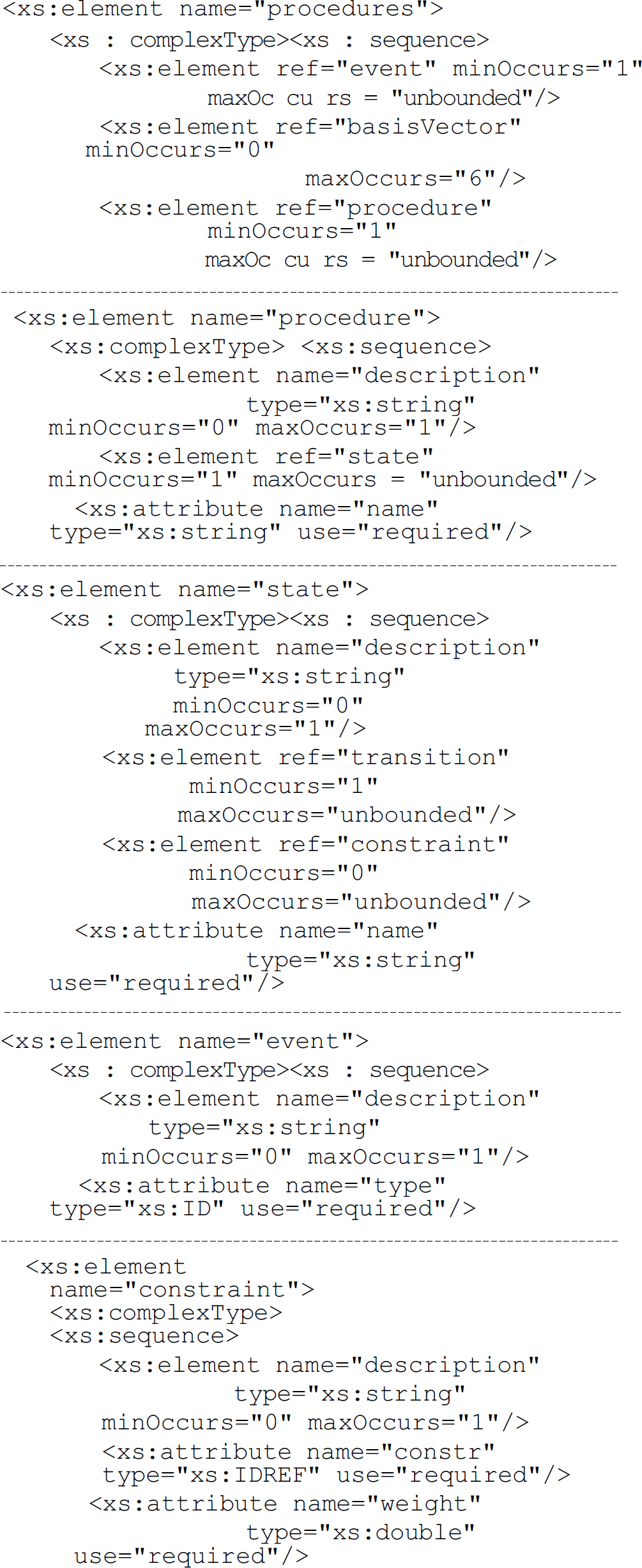
There may be a number of constraints defined for a certain state. Those are directly connected with the behavior of the system through the control algorithm. As examples of constraints, there may be a value which defines the level of compliance/stiffness of the robot, definition of virtual fixtures, etc. According to this specification schema, the Extensible Markup Language (XML), can now be used for task graph generation.

2.3. Task Graph Generation

There are three ways of generating a task graph:

i)

GUI - using a graphical interface that relies on the system structure and the specification file, see Fig. 2.

Fig. 2.

Graph generation for a surgical task using a simple GUI: for each state, a number of events are specified. In addition, the user can define a set of preferred directions and their magnitude as well as define the type of sensor for each primitive.

ii)

Learning - in (Hundtofte et al, 2000), it was shown how a simple language for modeling of multiple human-machine cooperative tasks can be designed. The underlying assumption was that a task is composed of gestemes - small component actions which are supported by the system. These are then be combined to generate task graphs on-line by recognizing users' actions,

iii)

Directly specifying the XML file.

2.4. Task Graph Execution

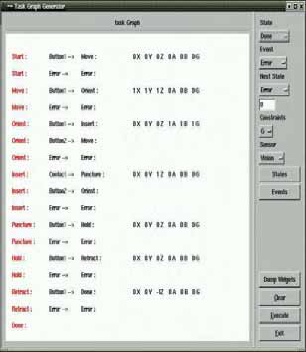
The task graph manager, see Fig. 1, configures the task with its underlying structure given the task graph. When invoking the control system, the task graph manager is initiated with command line parameters specifying a text file produced during task graph generation. The text file is interpreted so that the tree structure is built. After the task manager has received a confirmation that the whole tree is successfully configured, the system can be run. The system is event based and the task manager either Fig. 3. XR4000 - the experimental platform.

Fig. 3.

XR4000 - the experimental platform.

2.5. Example Scenario

The experimental platform for evaluation of the above control strategies is a Nomadic Technologies XR4000 shown in Fig. 3. The robot has two rings of sonars, a SICK laser scanner, a wrist mounted force/torque sensor (JR3), and a color CCD camera mounted on the gripper (Barrett hand). The palm of the Barrett hand is covered by a VersaPad sensor as shown in Fig. 4.

Fig. 4.

The Barrett hand, VersaPad and Android sensors.

The Versa Pad was designed to be used as a touch pad on a laptop. It reports: i) a Boolean value if the pad is active (contact occurred), ii) the coordinates of the contact point, and iii) pressure at the contact point. On each finger link, a pair of Android sensors is placed reporting the pressure applied to it. In addition, there is one Android sensor on each fingertip. The wrist mounted JR3 force-torque sensor is here primarily used as a “safety-break”: if the contact occurs on the VersaPad's “blind” spot, it can still be detected by the JR3 sensor.

Let us now study a simple object grasping task. Here, the following primitives are used for modeling:

INITIALIZATION: set connections with sensors, prepare hand,

APPROACH: move the robot arm from a starting position to some position close to the object,

ALIGN: align the hand with the object,

GRASP: grasp the object, LIFT: lift the object,

DONE: report that the task was successfully performed,

ERROR: if an error is reported, either i) exit or ii) continue with the execution allowing the user to choose the next state.

Now, the pseudo XML representation is as follows:

The task space of the robot is defined by a set of basis vectors representing all Cartesian directions. These basis vectors are then used in each of the states to de- fine the preferred motion for the robot. For example, during the Approach, we are only interested to movethe robot close to the object and therefore it is enough to use translational degrees of motion. On the other hand, during the alignment, a high accuracy is neededand therefore all six degrees of freedom are controlled.

3. Model Based Pose Estimation and Tracking

In order to perform the Approach and Align steps presented above, pose of the object has to be estimated. Our pose tracking system employs the classical detect-match-update-predict loop, (Kragic, 2001). In general, the key problem to robust and precise object tracking are outliers caused by occlusions, cluttered background, specular reflections, shadows and texture. Approaches like condensation, (Isard & Blake, 1998), cope with outliers by taking a large number of sample hypotheses of the position of the tracked structure and a comparatively small number of edge measurements per sample. Our tracking system achieves robustness using a large number of measurements for a every pose hypothesis. The idea, similar to the ones proposed in (Drummond & Cipolla, 2000) and (Harris & Stennett, 1990), is to use an image motion model to account for motion between consecutive frames using normal displacements. Some of the objects commonly used in our experiments are shown in Fig. 5.

Fig. 5.

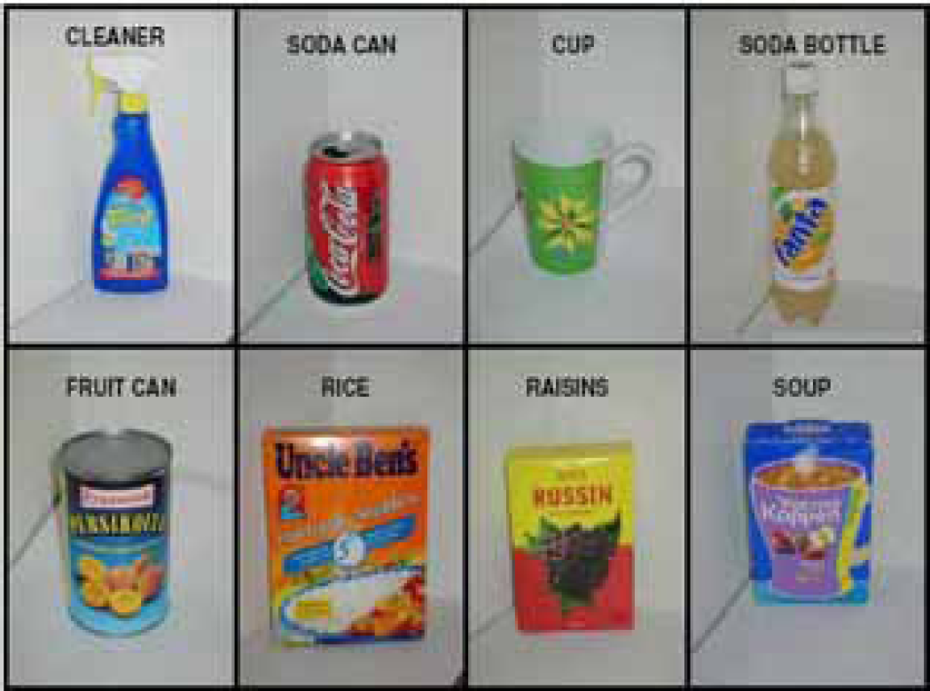
Example objects

Our approach relies on the estimation of normal flow for points (nodes) along lines and preserves the rigid structure of the object. As outlined in the introduction, the system is used for i) pose estimation, and ii) tracking. In our case, the basic differences between these two are:

• i)

Initial pose estimation retrieves the pose of the object at the beginning of the tracking (manipulation) sequence. Here, we assume that the initial guess is provided by an appearance based method or that a set of manual correspondences between the model and the object is available. The appearance based approach is briefly presented in Section 3.1. If, on the other hand, a set of correspondences is available, the iterative method proposed in (DeMenthon & Davis, 1992) is used. This step is followed by an extension of (Lowe, 1985) the nonlinear approach proposed in (Araujo et al, 1996).

ii)

Interframe pose change or pose tracking considers updating the pose of the object relative to the camera (or some other coordinate system) if there is a relative change in pose between these two. This is then used to track the pose of an object for cases where either (or both) camera and object are moving.

We have integrated both appearance based and geometrical models in our tracking system. After the object has been recognized and its position in the image is known, an appearance based method is employed to estimate its initial pose, (Kragic & Christensen, 2002).

3.1. Initialization

One of the problems to cope with during the initialization step is that the objects considered for manipulation are highly textured and therefore not suited for matching approaches based on, for example, line features (Vincze etal, 1999), (Wunsch & Hirzinger, 1997). The initialization step uses therefore the ideas proposed in (Nayar et al, 1996). During training, each image is projected as a point to the eigen-space and the corresponding pose of the object is stored with each point. Since the workspace of the robot is quite limited, a limited number of training images will suffice for most of the applications (Kragic & Christensen, 2002). At run time, the pose parameters are found as the closest point on the pose manifold. Now, the wire-frame model of the object can be easily overlaid onto the image. Since a low number of images is used in the training process, pose parameters will not accurately correspond to the input image. Therefore, a local refinement method employed for tracking (Section 3.2) is used for the final fitting, Fig.6.

Fig. 6.

Fitting stage and change in pose: The image on the far left shows the nearest training image. Its pose is used as the starting value for the fitting process. The absolute change in pose parameters is: AX=4mm, ΔY=8mm, ΔZ=138mm, Aa=23°, A/3=3°, A7=5°.

3.2. Pose Estimation

The system state vector is represented by position, orientation and object's velocity. Using the ideas proposed in (Drummond & Cipolla, 2000), normal flow along visible object features is used to find a geometric transformation of the object (relative change in pose) between two frames. Representing the pose of the object by a 4 × 4 homogeneous matrix X(R, t) and with an assumption of a small difference in pose between two adjacent frames, the relative change in pose is found as λX = Σ exp (g_iG_i) where gi represent the quantities of relative object motion observed in image and Gi are generators of a six-dimensional Lie group, each representing one of the six degrees of freedom of a rigid body.

3.3. Prediction and Update

The pose of the object is tracked over time using an a – β filter. Here, the pose of the target is used as measurement rather than image features as commonly used in the literature, (Wunsch & Hirzinger, 1997). This approach simplifies the structure of the filter which facilitates a computationally more efficient implementation.

3.4. Object Modeling

For most of the objects we want the robot to manipulate at this early stage, a simple polyhedral model will suffice. We have also integrated cones and cylinders in the system which allows us to deal with objects such as cups or plates. A model is constructed

A model is constructed from a set of primitives, see Fig.7. In the simplest case, the primitives are the apparent object edges used to model the objects by points, lines and polygons defined both in the camera (3D) and image (2D) space. In addition, surface creases, markings, or regular texture patterns (circles, ellipses) can easily be integrated in the model. Given the current pose of the object, a hidden primitive removal is performed using back face culling, (Foley et al, 1990). Assuming that the pose of the object changes a small fraction between frames, for optimization purposes, the visibility is not estimated in each frame

Fig. 7.

An object is represented with points, lines and polygons. A similar schematic overview is presented in [12].

4. Confluence of Parameters

We assume that the objects to be manipulated are placed on a table, shelf etc. In these situations, the background is fairly textured which, in the combination with textured objects, makes the process of feature detection relatively complicated. In terms of objects, surface patterns are ommonly irregular in terms of shape (letters, flowers, etc.) which does not allows us to generate simple features (lines, ellipses) on the surfaces. Since an object is defined as a set of related primitives, which are related both in 2D and 3D, the robust improvements for the algorithm can be obtained at two levels: i) Obtaining measurements directly in the image and elimination of outlying measurements in the image, and ii) Pose update in 3D and elimination of the outliers based on pose parameters.

4.1. Outliers rejection in 2D

A number of systems use tracking windows for each feature of the model which are warped along the main feature extension, (Wunsch & Hirzinger, 1997), (Vincze et al, 1999). After this, edgels are extracted inside the window and used to fit the feature geometry to the data. Consequently, all pixels inside the window have to be processed to obtain feature candidates making this approach time consuming. In our system, using the predicted pose of the object, the visible edges of the object are projected onto the image. A number of control points (nodes) is generated along the edges. Assuming a small change in pose between two frames, for each control point correspondences are sought for to find the strongest image gradient in the vicinity of the control point. Because of the aperture problem, only the perpendicular distance along the edge is measurable. Therefore, it is sufficient to choose one of the eight cardinal directions closest to the direction of the line normal, allowing image search in one-dimension rather than two-dimensions (i.e. linear vs. quadratic complexity in the search range). Contrary to Kalman filter based methods, our method does not require in particular the introduction of a state model, noise variance of the state and measurement models, which are often crucial factors. However, both background and object texture properties will introduce a significant number of false positives.

To improve the robustness with respect to the outliers, approaches such as RANSAC (Armstrong & Zisserman, 1995), factored sampling (Isard & Blake, 1998) and regulari-sation (Lowe, 1985) have been proposed. We have decided to use the estimated normal displacements and fit a line through those using the least squares line fitting proposed in (Deriche et al, 1992). After that, the new normal displacements are estimated as the perpendicular distance between a node and the new line, see Fig. 8.

Fig. 8.

2D outliers rejection: Using the predicted position of the edge, normal displacements are estimated, new edge position found and used to reestimate the normal displacements.

4.2. Outliers rejection based on pose estimation

In combination with the outliers rejection considering normal displacements, we have also used the idea shown in Fig.9. Given the predicted pose of the object and the model, we can easily predict the parameters of all the features in the image. In this case, if there is a considerable difference in angle between the predicted and estimated edge, the edge is disregarded during in the pose estimation step. This allows us to successfully cope with shadows commonly occurring in the vicinity of edges. In addition, there are cases where two of the model edges may get matched to the same line in the image. In this case, the edge for which the predicted position is closest to the detected edge is used for pose estimation.

Fig. 9.

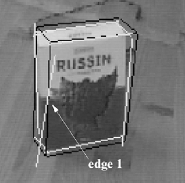
2D fitting process: visible edges are shown in black and new, detected in white. Edge number 1 is disregarded in the pose estimation step, due to the large difference in angle compared to the previous frame.

4.3. Gradient threshold

Assuming that there is a considerable difference between the object and the background, one-dimensional search usually gives us satisfactory results. To cope with small differences in gray-level values between adjacent pixels, a threshold is commonly used. Inadequate threshold may results in false positives and an unsuccessful matching step. An empirical evaluation has shown that an adequate initial value for the threshold regarding all the features is 20. During tracking, this value is changed based on the average gradient estimated for all the generated nodes on a feature by feature basis.

4.4. Feature stability

In certain cases, some of the edges will be difficult to detect. This may happen if the background and the object are similar in color or if there is no enough difference between different facets of the object based on he lighting conditions, pose of the object, occlusion, etc. Consequently, the “goodness” of a feature will vary during tracking. We have introduced a confidence measure attached to each of the features depending on the frequency with which the feature is found during a tracking sequence. The confidence value is used to weight the feature's responses during pose estimation.

4.5. Number of nodes along features

Determining the number of nodes generated along the visible object contours is also one of the important parts of the system. In a model based tracking system there will always be a trade-off between the time required to estimate one cycle and the provided accuracy in terms of pose. There are two parameters that determine the number of nodes: i) current velocity of the object (or the change in pose) - if the change in pose between the frames is significant, the number of nodes is kept low, and ii) the confidence measure of a feature - for features with high confidence, a smaller number of nodes are generated.

4.6. Color space

Commonly, gray-level images are used during this type of tracking. It is widely known that in some cases, the blue channel contains lots of noise and is often disregarded. We have decided to investigate the idea of how much the information from different channels can help us during tracking. The basic idea is to base the evaluation on the sum of the gradients along the visible object features C = argmax_C [J2v_x |VI(p) n_e|] where VI is the intensity (color value) gradient along the projected model edges, n_e is the edge normal, p is a point along the edge e and V_X are the visible edges of the model given the current pose X(R, t). Considering the objects shown in Fig.5, we have estimated this value during a number of successful tracking sequences. During all the sequences the objects were placed on a table, see Fig. 12. The plots for each of the objects are shown in Fig. 10. It can be seen that depending on the object properties, different channels gave different values for C. Consequently, the channel providing the highest value is chosen for tracking.

Fig. 10.

Average gradient plots for objects shown in Fig.5 using different color channels.

Fig. 11.

Error in pose when the object was tracked using different color channels. Here, the pose estimated from the red channel is used as the reference since it almost perfectly corresponds to the ground truth value.

Fig. 12.

An example sequence where First row) the initial system without the improvements is used and where Second row) the system with the improvements proposed in Section 4 is used. The last two rows show the estimated pose and their difference for these cases. Here, grad stands for the basic system, while WL denotes the improved system (see Section 5.2 for detailed explanation).

5. Experimental evaluation

The following sections present the experimental evaluation of or model based tracking system with the improvements proposed in the previous section. The system runs at frame rate on a standard Pentium PC.

5.1. Color space

The idea of using the channel giving the maximum average gradient was exploited in the following experiment where the system tracks a package of rice. Fig. 11 shows the difference in estimated pose parameters for each of the R,G,B channels. Here, the pose estimated from the R channel is used as the reference since it almost perfectly corresponds to the ground truth value. We will further investigate this basic idea for each of the features separately.

5.2. Tracking

Fig. 12 shows an example tracking sequence. The first two rows show a few images from the tracking sequence where the first row shows a unsuccessful and the second row an successful run. The estimated pose is overlaid in white. Here, the relative change in pose between the initial and the las frame is: ΔX=30mm, AY=10mm, ΔZ=30mm, Aa=8°, A/3=45°, A7=35°. The goal here was to show how the system with the improvements proposed in the previous section copes with the significant changes in rotation. In the case of the first row, we have used the approach as proposed in (Drummond & Cipolla, 2000) where normal displacements are used for pose estimation. It can be seen that during the rotation, when one of the back faces comes to front, the tracker looses the object. The reason for this is that two nearby edges, belonging to that surface, get incorrectly matched. This does, however, not happen in the case of the improved system since because only the nearest edge is matched, and the other one is disregarded during pose estimation. The last two rows show the plots of each of the pose parameters as well as the error between them.

5.3. Local Fitting

Fig. 13 shows an example of the fitting stage. The two main differences between the examples are: i) the value of the minimum gradient required to estimate the normal flow as presented in Section 4.3, and ii) the ouliers rejection as presented in Section 4.1 and Section 4.2. The images in the upper row show an example of an unsuccessful fitting where only normal displacements are used in the pose estimation process. In addition, the thereshold value for which a point is detected as edge was set to 10. This value was to low for this type of object and the background. In the second case (lower row), we have changed the gradient threshold to 20 and used outliers rejection as proposed in Section 4.1 and Section 4.2. The figure demonstrates a successful fitting step.

Fig. 13.

Two examples of fitting where the differences are i) the value of minimum gradient required to estimate normal displacements as presented in Section 4.3, and ii) the rejection of outliers using the ideas proposed in Section 4.1 and Section 4

6. Conclusions

In this paper, a simple framwork for design of fetch-and-carry tasks was presented. The current system consists of three levels: i) task graph modeling and generation, ii) task graph execution and iii) low-level implementation of control primitives. The motivation for such a design is that the complex tasks we consider are commonly repetitive and sequential in nature consisting of simple steps. In the current system, the transitions between these steps are driven by sensory or predefined pose information. Consequently, complex tasks are modeled using a set of basic steps or primitives where each primitive defines some basic type of motion (e.g. translational motion along a line, rotation about an axis, etc.). One example run is shown in Fig. 14.

Fig. 14.

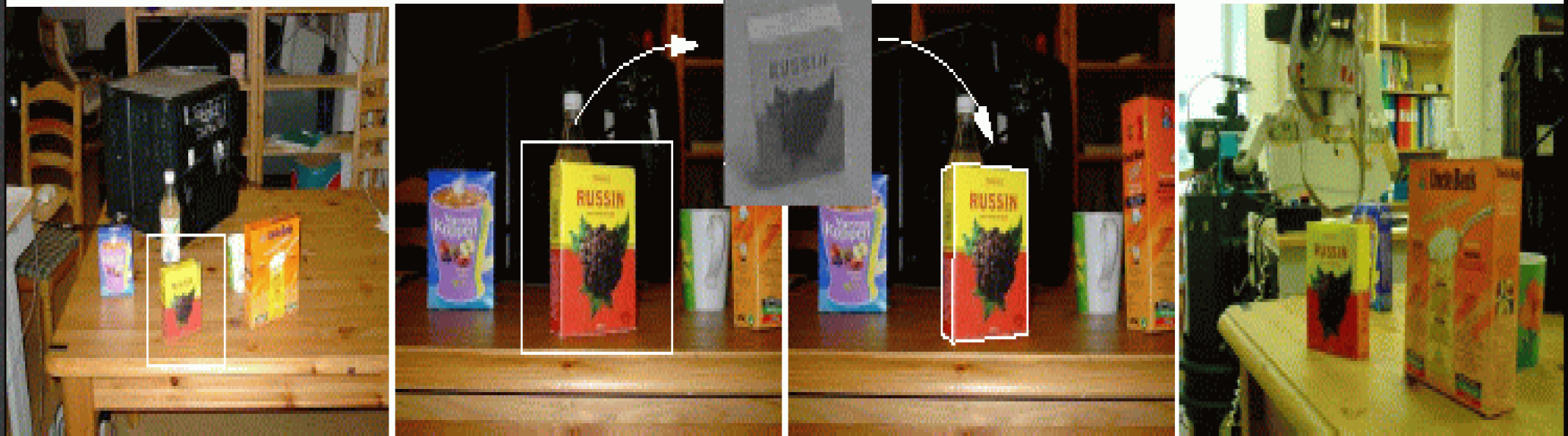
After the object is recognized, 2D tracking is used to approach the object and followed by a local fitting to estimate the current pose of the object. After that, grasping is performed.

We have also presented a model based tracking system and discussed its performance for cases of moderately textured objects in an everyday environment. The system relies on a simple geometrical model of the object to estimate its position and orientation in camera/robot coordinate system. Our approach integrates a number of ideas proposed in similar systems to achieve the robustness required for real-world applications. The main objective of the paper was the consideration of the different parameters and their effect the system's performance. One of the key problems that has to be addressed in a tracking system are outliers. Textured background, shadows, occlusions, etc. will produce edges in the close proximity of the model edges. These are a particular problem for the traditional least-square fitting method used at this stage. Our future work will therefore consider the use of RANSAC that differs from the conventional least squares techniques as a small subset of data is used to estimate feature parameters. A problem that can occur for objects of simple geometry (boxes, cups) is that in some frames the number of detected features will give rise just to some of the pose (velocity) parameters. We will further investigate how, in this case, just the adequate pose parameters can be updated. Finally, our ultimate goal is to regain tracking after it has been lost. Our idea is to integrate the appearance based method as the one used during the initialization step to allow continuous tracking and achieve a fault tolerant system.