Design and Analysis of an Underwater White LED Fish-Attracting Lamp and its Light Propagation

Abstract

Light emitting diodes (LED) are a new source for replacing traditional light sources including under water illumination. As traditional underwater light sources operate under a radiative transfer model, the luminous intensity is dispersed evenly at each emission angle, with the scattering factors included in the attenuation coefficient. By contrast, LED light sources are characterized by being highly directional, causing underwater luminous energy to vary with different emission angles. Thus, the traditional theory of underwater optical transfer becomes inapplicable when an underwater LED lighting module is designed. Therefore, to construct an underwater transfer model for LED light sources, this study employed the average cosine of the underwater light field, the method for light scattering probability, the LED luminous intensity distribution curve (LIDC) and axial luminous intensity. Afterwards, an underwater LED fish-attracting lamp was designed. Experimental results showed that, compared with the simulation values, the luminous intensity of the underwater LED lighting module at all emission angles had a percentage error of less than 10%.

1. Introduction

Considering the current context of low-carbon economy (LCE), replacing high energy consuming high-intensity discharge (HID) lamps with LED lights, which are highly energy-efficient, has become an inevitable trend, especially in the field of underwater illumination. HID light sources are full of toxins and fail to reach current standards in the face of increasing environmental awareness. Additionally, they cover both visible and invisible optical wavelengths and most of the luminous energy is concentrated at the red waveband between 600 and 700nm. According to Rayleigh's scattering formula, when light is scattered in such a medium as water, luminous intensity (I) is inversely proportional to the fourth power of the incident wavelength (λ) [1]. In other words, the shorter a wavelength is, the harder it is for luminous intensity to attenuate within the scattering environment. Therefore, HID light sources have low efficiency underwater and must use more energy to achieve the required illumination. However, the underwater illumination zone does not increase proportionally with the power increase. Accordance to the Lambert-Beer Law, when incandescence power increases from 15W to 6kW, the consumed energy increases 400-fold, whereas the underwater illumination zone increases only 7.8-fold [2]. By contrast, LED lights are highly directional and efficient. Their light beams are focused on the designated zone by the lenses at different emission angles; consequently, energy waste is reduced. Furthermore, the highly directional light emission of LEDs differs from the radiative emission of traditional light sources. Thus, traditional methods cannot be used to design LED lights. Instead, the parameters involved must be analysed, such as the transfer model for underwater LED beams, the emission angles and light intensity of LED light sources.

Ocean engineering and fishery technology often involve underwater operations, where underwater illumination is indispensable. Different underwater operations have different illumination requirements. Some require mobile illumination, others need a proximate short-range illumination and still others call for long-range guidance illumination. Despite these needs, underwater optics is rarely studied in the field of LED optical design. This is because underwater illumination frequently focuses only on illumination distance and illuminance, and such questions as light types and uniformity are neglected. As indicated by the Lambert-Beer Law, an underwater light typically attenuates under the light transfer model, meaning that attenuation of the transferred light is defined by an exponential function. However, the measured value of light intensity attenuation often deviates slightly from a theoretical value. This deviation is primarily caused by some simplified assumptions in the Lambert-Beer Law prior to its establishment. For example, it is assumed that the incident lights, parallel to one another, belong to a single waveband and that the medium is a uniform, non-scattering system [3]. Although this law is significantly flawed in practical application, it can rapidly estimate the underwater attenuation coefficient, thereby predicting the illumination zone for each depth. However, for water bodies with high scattering properties, such as rivers, seas and lakes, Lambert-Beer's underwater light transfer function causes significant errors. Furthermore, all the obtained information about underwater light transfer is nothing but an attenuation coefficient. As a result, how the light beam is actually transferred in the water body cannot be described effectively [4]. In recent years, the Monte Carlo method for ray tracing has been commonly employed to analyse the model for underwater light transfer [5-6]. Based on the relationship between any object and its environment, this technique simulates the interaction and transfer process by tracking the transfer path of each ray. Dependent on the relationship between objects, numerous random numbers and iterations are used during the simulation process until the calculation results converge on the same trend. After that, the substantial parameters of the water body and the model for underwater light transfer are identified. Kirk (1991) and Haltrin (1997) used the Monte Carlo concept to develop a method for the average cosine of the light field, which was combined with various kinds of underwater optical properties and scattering probabilities, to examine underwater light transfer [7-8]. By means of the Monte Carlo method, Adams et al. (2002) simulated the scattering process of underwater light beams and determined the light-field distribution of underwater light sources [9]. However, none of the above studies examined LED light sources in an underwater environment. By combining LED luminous intensity distribution curves (LIDC), axial light intensity and a model for light transfer attenuation in space, Guttsait (2007; 2009) studied the LED lighting module to quantify its long-distance illuminance, uniformity and efficacy [10-11]. Nevertheless, Guttsait did not explore the optical properties of the underwater LED lighting module. Therefore, by using the method for the light-field average cosine to integrate the luminous intensity distribution curves (LIDC) and axial luminous intensity of LEDs, we constructed an underwater transfer model for LED lights. Moreover, this study explored the light-field distribution and effective illumination distance of the underwater LED lighting module at various emission angles. Finally, an underwater LED fish-attracting lamp was designed and manufactured in compliance with the underwater transfer model for LED lights. Meanwhile, underwater optical measurements were performed. To be more specific, the properties and relevant parameters of underwater light-field distribution were measured at different emission angles to provide a reference for future studies of underwater LED optics.

2. Analysis of Underwater Light Field of LEDs

2.1. Light Transfer and Scattering

Mobley (1994) stated that when a single-band light beam is incident on an extremely small water body, some of the incident energy is absorbed and some is scattered as it passes through the medium, with the rest of the luminous energy continuing in the original direction [12]. Consequently, when a light beam is transferred underwater, its luminous energy attenuates because of absorption and scattering. This is true of a traditional underwater fish-attracting lamp, whose light beams are radiated in all directions, so its luminous intensity is dispersed evenly at each emission angle (Figure 1(a)), with the scattering factors included in the attenuation coefficient.

Figure 1.

Traditional HID and LED light beams are transferred underwater.

Formula (1) defines the Lambert-Beer underwater transfer model for traditional light sources, where I_L is the intensity at transfer distance L, I₀ is the intensity at the light source and c is the overall attenuation coefficient, including absorption and scattering coefficients. By contrast, LED light sources are highly directional and planar, causing the underwater luminous intensity to vary at different emission angles (Figure 1(b)). Because of this phenomenon, the established theories about traditional light modules cannot be applied when underwater LED illumination is analysed.

$I_L=I_0\exp \left[-cL\right]$

(1)

The average cosine of an underwater light field, which means the average cosine of the positive angle in the light-emitting direction, primarily quantifies the angular distribution of the underwater light field. It also provides the distribution value for each emission angle of the underwater light field. Traditional lamps are radiative light sources, having the same average cosine measured at the same distance but at various angles. By contrast, LED light modules are highly directional and planar, having different average cosines measured at the same distance but at different angles. In practice, significant scattering of the light beam occurs because of the particles being suspended in water. As a consequence, when a light beam is transferred in water, the light field distribution changes significantly with various travel distances and scattering events. In other words, the longer the transfer distance is and the more times scattering happens, the more obvious the diffuse features of the light field are on the outside of a directional light source. For highly directional LED lighting modules, when collimated beams are transferred in water, the initial beams in identical travel directions have an average cosine of 1. As the transfer distance continually increases, scattering probability also becomes greater and the average cosine decreases, eventually approaching 0. That is to say, the light field approaches a state of diffuse distribution. Supposing that a collimated beam is travelling through the water at a nadir angle θ₀ and after scattering it obtains a scattering angle α, the scattered light disperses on a cone at an angle α to the original incident direction, as shown in Figure 2.

Figure 2.

Schematic diagram of how the scattered light disperses.

After those particles with a scattering angle α are scattered, the average cosine is obtained below:

$\begin{array}{c}\bar{\mu }\left(\alpha \right)=\overline{\cos \theta }\\ =\frac{1}{2\pi }{\displaystyle \underset{0}{\overset{2\pi }{\int }}\left(\cos {\theta }_0\cos \alpha +\sin {\theta }_0\sin \alpha \cos \phi \right)d\phi }\\ =\cos {\theta }_0\cos \alpha \end{array}$

(2)

Once the average cosine of the scattering angle α is calculated, the angle of 0→π is divided into N segments of equal size and the average cosine of the random number α is obtained below:

$\begin{array}{l}\bar{\mu }\left(\alpha ,0\to \pi \right)=\bar{\mu }\left({\alpha }_1\right)Y_1+\bar{\mu }\left({\alpha }_2\right)Y_2\\ +\wedge +\bar{\mu }\left({\alpha }_i\right)Y_i+\wedge +\bar{\mu }\left({\alpha }_N\right)Y_N ={\displaystyle \sum _{i=1}^N\bar{\mu }\left({\alpha }_i\right)Y_i}\end{array}$

(3)

where α_i is the mid-point of the ith angular segment observed and Y_i is the probability that the particle falls on the ith angular segment after scattering. Based on the phase scattering function, Y_i is defined as:

$Y_i=2\pi \beta \left({\alpha }_i\right)\sin {\alpha }_i\mathrm{\Delta }\alpha$

(4)

where β(α_i) is the phase scattering function.

From formulas (2), (3) and (4), the following formula is obtained:

$\begin{array}{c}={\displaystyle \sum _{\alpha =0}^{\pi }2\pi \beta \left(\alpha \right)\cos {\theta }_0\cos \alpha \sin \alpha \mathrm{\Delta }\alpha }\\ \bar{\mu }\left(\alpha ,0\to \pi \right)={\displaystyle \sum _{i=1}^{N}2\pi \beta \left({\alpha }_i\right)\cos {\theta }_0\cos {\alpha }_i\sin {\alpha }_i\mathrm{\Delta }\alpha }\\ =\cos {\theta }_0{\displaystyle \underset{0}{\overset{\pi }{\int }}2\pi \beta \left(\alpha \right)\cos \alpha \sin \alpha d\alpha }\end{array}$

(5)

The integral of the above formula defines the average cosine below [13]:

$\bar{\mu }\left(\alpha ,0\to \pi \right)=\cos {\theta }_0\times \bar{\mu }$

(6)

Formula (6) shows the change in the average cosine after the light beam with an emission angle of θ₀ is incident upon the water and undergoes one scattering event. Therefore, given that the average cosine of the incident light is μ₀, the final average cosine after the beam has undergone n times of scattering is:

$\bar{\mu }\left(n\right)=\overline{{\mu }_0}\cdot {\bar{\mu }}^n$

(7)

Evidently, as the light beam travelling underwater scatters again and again, its average cosine will decrease constantly. Moreover, the attenuation rate of the average cosine depends on the scattering phase function β(θ). The travelling light beam will nearly be diffused after scattering a number of times. Consequently, the smaller the average cosine, the more times the light beam is scattered and the closer the travelling beam is to the state of diffusion. In addition, the scattering probability of the light beam travelling underwater can be calculated. Supposing that the light travels underwater for a distance L, its scattering probabilities are given by P(0), P(1),P(2), …P(n). P(0) represents no scattering P(1) means one scattering event and P(2) means two scattering events. Furthermore, P(0), which means no scattering is defined as:

$P\left(0\right)=\exp \left(-bL\right)$

(8)

where b is the scattering coefficient.

P(1), which means the probability of only one scattering event after a light beam travels the entire path L, is defined as:

$P\left(1\right)={\displaystyle \underset{0}{\overset{L}{\int }}\exp \left(-bL\right)bdl=bL\exp \left(-bL\right)}$

(9)

Therefore, P(n), which means the probability of n scattering events after a light beam travels the entire distance L, can be defined as:

$P\left(n\right)=\frac{{\left(bL\right)}^n}{n!}\exp \left(-bL\right)$

(10)

Figure 3(a) and 3(b) show the scattering events undergone by light beams, which travel 20m in different water bodies. According to Kirk (1999) [13], a scattering coefficient b=0.059 indicates a slightly turbid water body, b=0.321 indicates a mildly turbid water body and b=1.719 indicates a highly turbid water body.

Figure 3.

The relationship between scattering probability and scattering times for a light beam travelling 20m in different water qualities.

Figure 3(a) shows that in different water qualities, light beams travelling the same distance undergo vastly different numbers of scattering events. For a beam travelling 20m in slightly turbid water, 16% of the photons do not scatter, but 29% and 27% experience 1 and 2 scattering events, respectively. In other words, over 70% of the light beams experience no more than two scattering events during the entire transfer process and the rest of them scatter no more than 4 or 5 times. In mildly turbid water, most light beams scatter between 5 and 15 times. However, in highly turbid water, the results differ completely. As indicated by Figure 3(b), the maximum amount of scattering in highly turbid water is approximately 90. Moreover, as shown in Figure 4, the average cosine varies with the times of scattering; namely, the scattering process has a significant effect on the average cosine, especially the first 15 incidences. After the collimated beam scatters 5 times, its average cosine declines to 0.6 and then it declines below 0.3 after 15 scattering events. Once the number of scattering events exceeds 50, the average cosine is close to 0, indicating that the light beam is diffused. That is to say, when a light beam travels for more than 20m in a turbid water body, almost all its luminous energy has already been scattered away. Therefore, analysis of underwater light scattering reveals how a light beam is transferred and how its luminous intensity attenuates.

Figure 4.

The relationship between the average cosine and scattering times.

Based on formula (7), which defines the average cosine of a light beam after it undergoes n scattering events and formula (10), which defines the scattering probability of a light beam after it travels a limited distance L and undergoes n scattering events, the average cosine μ(L) of an underwater beam can be obtained after it travels the distance L:

$\bar{\mu }(L)={\displaystyle \sum _{n=0}^{\infty }{P}_L\left(n\right)\cdot \bar{\mu }\left(n\right)}$

(11)

When the attenuation coefficient is imported into the scattering factor, the attenuation function will vary with the travel distance L, scattering times n and the absorption coefficient a, as defined below:

$C\left(L\right)=\frac{a}{\bar{\mu }\left(L\right)}$

(12)

where a is the absorption coefficient of the light beam and C(L) is the attenuation function at any random travel distance L.

Finally, the transfer formula for the underwater light beam with a scattering function is given by:

$I_L=I_0\exp \left[-C\left(L\right)\cdot L\right]$

(13)

where I_L is the luminous intensity at travel distance L, I₀ is the light source intensity and C(L) is the overall attenuation coefficient.

2.2. LED Light Source Properties

As the most important characteristic of LED light sources, LIDC includes the relationship between emission angles and axial light intensity distribution. From a traditional light source, or a point light source, light is radiatively transferred; thus, its luminous intensity is identical at different angles. By contrast, an LED light source is directional and planar; therefore, its luminous intensity varies with different emission angles. As for a Lambertian light source, each emission angle and its luminous intensity can usually be expressed through Formula (14) [14]. Furthermore, the emission angle is defined as a corresponding angle with 50% of the axial luminous intensity.

$\{\begin{array}{c}I\left(\theta \right)=I_{ALI}{\cos }^m\left(\theta \right)\\ m=\frac{-\ln 2}{\ln \left(\cos {\theta }_{0.5}\right)}\end{array}$

(14)

In the case of different LED LIDC, Formula (14) can be used to obtain the axial luminous intensity (IALI). The illuminance E of an LED light source at any point underwater can be obtained by integrating Formula (13), i.e., the model for underwater light transfer and Formula (14), i.e., the scattering function. Therefore, selecting an appropriate LIDC to match the water's turbidity is crucial to light module design.

$E\left(\theta ,l\right)=I\left(\theta \right)\cos \theta \cdot \exp \left[-C\left(L\right)\cdot L\right]$

(15)

The above Formula (15), which combines Formulas (13) and (14), shows that based on the properties of LED light sources, this study integrates the average cosine of the light field and the method for light scattering probability. Next, concerning a directional light beam transferred underwater, this study analyses its scattering scenarios at different distances and the change in angular distribution of its light field. Thus, the authors have constructed a transfer model for the underwater LED light source.

3. Design and Analysis of underwater LED Fish-attracting Lamp

Traditional light sources belong to point sources, with equal luminous energy at all emission angles, which usually renders illumination distances proportional to illumination zones. In other words, the farther a light beam is transferred, the larger its illumination zone is. By contrast, LED lights are directional and planar, so luminous intensity varies with LIDC at different emission angles. While the illumination zone of a traditional light source can be estimated based on the illumination distance in one single direction that of an LED light cannot. Therefore, in designing an underwater LED light source, the authors had to consider the relationship between emission angles and illumination zones of different light sources. Take underwater fish-attracting lamps as an example. If the illuminance of 10 lux visible to the fish eye is set as a standard, a single LED light source cannot provide sufficient illuminance. To solve the problem concerning insufficient illuminance, this study designed an LED array light source. The illuminance E of the LED array light source at any point underwater can be expressed mathematically as:

$E_{total}\left(\theta ,l\right)={\displaystyle \sum _i{E}_i\left({\theta }_i,l_i\right)}$

(16)

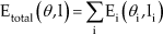
where E_i is the illuminance of the ith LED, with a corresponding angle θ_i and a distance l_i. Formula (16) can be used to show the light field distribution of the LED array in its corresponding environment.

To analyse underwater LED fish-attracting lamp, this study used different LED arrays (1×1, 1×2, 1×4, 1×8, 1×12 and 1×18) with a luminous efficacy of 90lm/W and simulated their maximum illuminance (L_max) and illumination zones (V) at different emission angles in a 220m long, 10m wide and 3m deep towing tank. An illuminance meter (Konica Minolta model T-10) is used to measure the underwater distribution of light intensity. To reduce the effect of the water body's attenuation coefficient on the simulation results, high-intensity discharge (HID) fish-attracting lamps were first placed in the towing tank to measure the value of the underwater light transfer. Then, the Lambert-Beer model for underwater light transfer was employed to calculate the overall attenuation coefficient in the towing tank. Figure 5 shows the illuminance of the traditional HID fish-attracting lamp measured at each illumination distance 2m underwater. As indicated by Figure 5, the measurements of the underwater HID fish-attracting lamp satisfy the Lambert-Beer model for underwater light transfer; namely, the lights display exponential attenuation. Meanwhile, the overall attenuation coefficient c=0.217 was obtained through the regressive analysis method. Furthermore, when a light beam is incident upon an extremely small water body, no inelastic scattering occurs and nor do the wavelengths of photons change during the scattering process. Based on the law of conservation of energy, the attenuation coefficient of the transferred beam includes the absorption and scattering coefficients. If the absorption coefficient of pure water involving visible light wavebands is 0.1 [15], the scattering coefficient of the water body in the towing tank used for this experiment can be estimated at 0.117. We designed and simulated underwater LED array lighting modules using Matlab software.

Figure 5.

The illuminance of traditional underwater HID fish-attracting lamp measured at each distance 2m underwater.

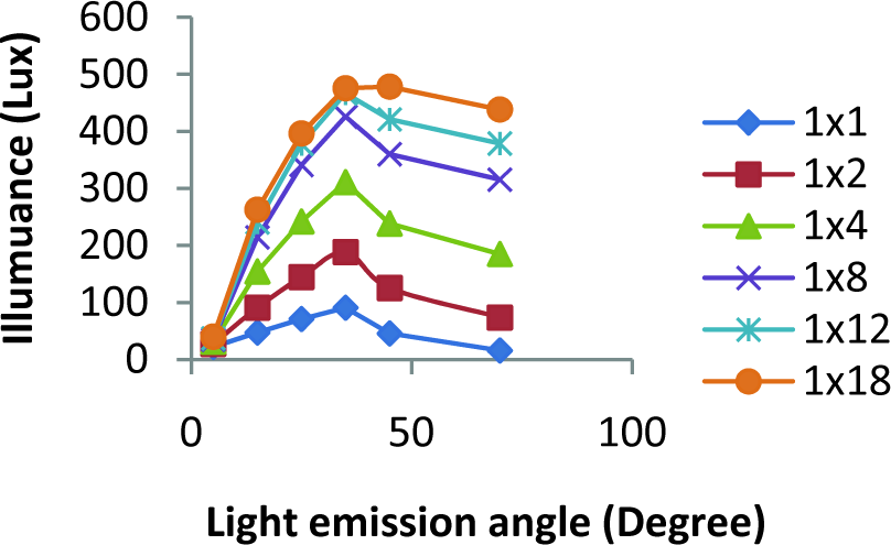
Take an underwater LED fish-attracting lamp for example. Its illumination zone is the volume of the illuminated area with an illuminance greater than 10 lux after light is emitted from the light source. As shown in Figure 6, the simulation results reveal the illuminances of LED array light sources with different emission angles and different numbers of arrays, which were placed 10m or 20m away from a target. For a single LED light source at an emission angle of 5°, even at the longer travel distances, even up to 20m, its illuminance remained 35 lux. However, because the emission angle was too small and the illumination zone was too narrow, identifiable illuminance could not be achieved. For a LED light source with an emission angle of 70°, its light beam appeared to diffuse at 20m away from the source and the illuminance was only 0.28 lux, being too meagre to distinguish objects or to entice marine creatures. Figure 7 is the simulated light field distribution diagram of a 1×18-array LED light source at different emission angles underwater. At small emission angles, such as 15° and 25°, the increased number of arrays obviously enhanced its illuminance. Its luminous intensity was high enough to reach a longer distance because of the low scattering probability of a light beam with a smaller emission angle, as shown in Figure 7(a) and 7(b). However, as the emission angle of the LED light source gradually increased, for example, to 70°, the illuminance no longer rose significantly with the added LED arrays, as shown in Figure 6. Consequently, as the emission angle became larger, large amounts of luminous energy would meet too many scattering media during the transfer process, with scattering probability increased. The above results show that the effective illumination distance of luminous energy decreases as its emission angle becomes larger, as shown in Figure 7(c) and 7(d).

Figure 6.

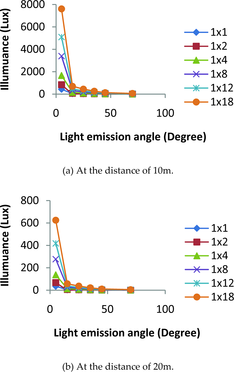
The illuminance of LED light sources with different numbers of arrays and at different emission angles.

Figure 7.

The simulation results of underwater light field distribution involving a 1×18-array LED light source at different emission angles.

Figure 8 shows the change in the illumination zone of an LED array. When its emission angle was 5°, the illumination zone was too narrow because of the small emission angle. Thus, the illumination zone could not be enlarged despite a continual increase in the number of LED arrays. However, the illumination zone could be significantly enlarged if its emission angle was gradually increased. Additionally, the maximum illumination zone of a 1×4-array LED light source with an emission angle of 35° was 141.78m³ and its illuminance at a distance of 20m was 4.78 lux, as shown in Figure 6 (b). When the emission angle gradually increased, its illumination zone rapidly decreased. At 70°, its illumination zone dropped to 45.85m³ and its illuminance at a distance of 20m rapidly declined to 1.10 lux. A similar pattern happened to a 1×18-array LED light source, whose maximum illumination zone was 381m³ at 35° and whose illuminance at 20m was 21.55 lux. However, at 70°, its illumination zone declined to 264m³ and its illuminance at 20m decreased to 4.95 lux. However, after the number of LED arrays grew, the light travel distance lengthened because of increased luminous energy and the illumination zone expanded, too. Therefore, based on the above analysis results of the underwater transfer function concerning the LED array light source, an emission angle of 35° produced the optimal travel distance and illumination zone in a water body with average quality.

Figure 8.

The illumination zones of underwater LED fish lamps at different light emission angles and with different numbers of LED arrays.

Regarding the design of underwater LED fish-attracting lamps, the LED light source employed in this study was an XLamp XT-E Royal Blue, manufactured by CREE, with a light-emitting efficacy of 90lm/W and a maximum driving current of 1A. According to the above analysis results, light-absorbing lenses with an emission angle of 35°and a 1×12-array LED were adopted as the production parameters so that the underwater LED fish-attracting lamp might acquire the maximum travel distance and illumination zone in the towing tank, which had an absorption coefficient of 0.1 and a scattering coefficient of 0.117. The prototype of the LED fish-attracting lamp is shown in Figure 9.

Figure 9.

The prototype of the underwater LED fish-attracting lamp constructs by 1×12 chip on board LED array.

4. Measurement and Discussion

The authors constructed the transfer model for the underwater LED fish-attracting lamp by employing the average cosine of the light field, the method for light scattering probability, the LIDC and the axial luminous intensity of LEDs. Thereafter, we designed an underwater, high-intensity LED array light source and conducted an experiment on the measurement of long-distance light transfer in a towing tank, which belonged to the Department of Systems & Naval Mechatronic Engineering, National Cheng Kung University. In accordance with the measurement results, when a light beam is transferred underwater, scattering events primarily occur during the time that photons collide with particles. In other words, when a light beam travels underwater, the number of collisions is an important factor affecting the occurrence of scattering. If the scattering factor increases, the number of collisions that a beam must undergo before it reaches its goal also increases. Therefore, the scattering factors of different water bodies influence the distance that a beam travels underwater, especially for surface light sources.

Regarding the optical measurement of the underwater LED array lamp, which is a highly directional and planar light source, the measurement configurations were fully compatible with its optical properties, as shown in Figure 10. The illuminances at different distances and positions were measured to verify its light field distribution diagram. Additionally, to reduce the error caused by its deviated measurement point, it was placed 2m underwater and measuring was started 4m away from it. To be more specific, an emission degree of 0° at the light source was used as the axial line and a measurement line was drawn at an interval of 1m in both directions. Horizontally, starting at 4m away from the light source, the endpoint of each metre served as a measuring point and the illuminance at each point was measured. The measurement results of the light field distribution concerning the underwater LED array light source are shown in Figure 11. First, long-distance illuminance was measured along its axial line. As shown by the Figure 11, the beam transfer attenuation was similar to that of a traditional lamp. Next, illuminance was measured on either side 1m away from the longitudinal axis, with line (b) in Figure 11 showing the attenuation curve in both areas. Theoretically, the illuminances on both sides of the light source should be equal; however, in fact, the illuminance on the left side was greater. This disparity was primarily caused by overlapping of the sub-beams within the LED array light source. This phenomenon became more obvious when the beam was closer to the light source. Therefore, the measurement points on different sides near the light source were prone to produce asymmetric results. Long-distance illuminances were also measured on both sides again at 2m away from the axial line, as shown in Figure 11 line (c). The figure shows that the illuminance at 4m to 6m away from the light source initially grew before declining gradually. This trend was caused by the difference in LIDC between LED and traditional lamps. As the LED light beam is not transferred radiatively and is limited by emission angles, the farthest area outside of the light field is incredibly dark, as shown in Figure 11 line (b). Furthermore, as the distance increases, illuminance initially increases before attenuating gradually to zero.

Figure 10.

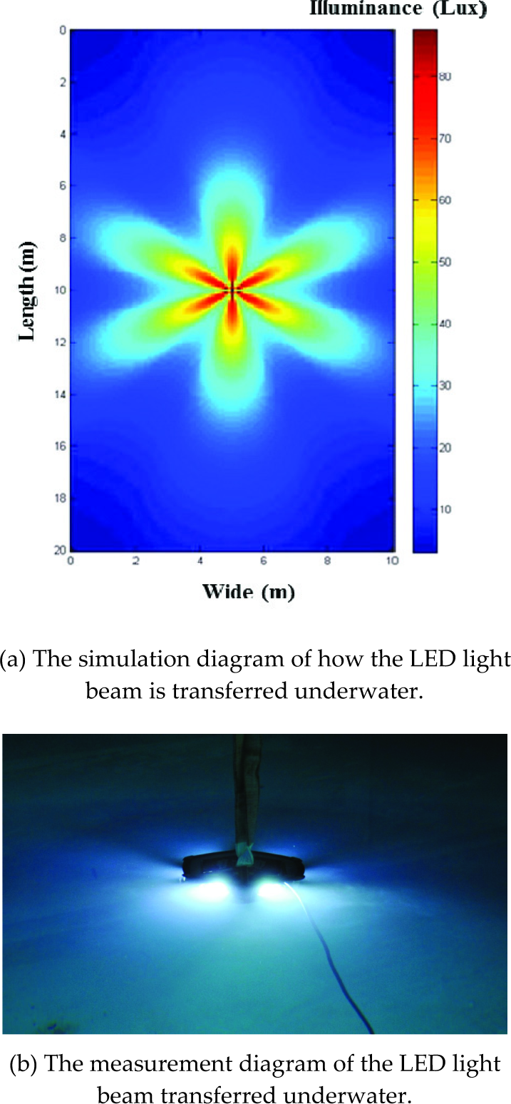
The simulation and measurement diagrams of the underwater LED light beam.

Figure 11.

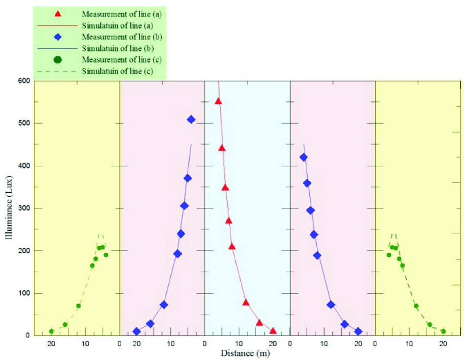
The light field distribution of the underwater LED fish-attracting lamp was measured and simulated.

In general, after the illuminance and the simulation value at each measurement point were compared, it was discovered that most measured values were smaller than the simulation values, with a total error of approximately 10%. However, when the illuminance error at the boundary between the dark and bright sides of the light field was excluded, the difference between the simulation value and the measured value was less than 1 lux. Therefore, the model for underwater LED light transfer presented in this study can be used instead of the theory about traditional underwater light transfer when an underwater LED array lamp is designed.

5. Conclusions

This study constructed the model for underwater LED light transfer by employing the average cosine of the light field, the method for light scattering probability, the emission angles and the axial luminous intensity of the LED light source. In addition to establishing an underwater LED fish-attracting lamp, this study successfully presented its underwater light field distribution and analysed its illuminance, as well as illumination zones at different emission angles. The simulation results of underwater light transfer showed that to obtain a longer travel distance, a smaller emission angle is required. However, to achieve a bigger illumination zone, an LED light source with a larger emission angle is not necessarily better; instead, it depends on the absorption and scattering coefficients of the water body. The experimental results show that in general water bodies, the maximum illumination zone of a 1×18-array LED light source with an emission angle of 35° was 381m³ and that the illuminance at 20m underwater was 21.55 lux. Designed under the model for underwater LED light transfer, the LED array lighting module had a percentage error of less than 10% when the luminous intensity at each emission angle was compared with the simulation value. Therefore, this design method can be used not only to evaluate the illumination distance and zone of an LED lighting module in various underwater environments, but also to serve as the foundation of future studies on designing underwater LED fish-attracting lamps.