Sage Journals: Discover world-class research

Abstract

Efficient control schemes are required for effective cooperation of robot teams in a mobile wireless sensor network. If the robots (resources) are also in charge of executing multiple simultaneous missions, then risks of deadlocks due to the presence of shared resources among different missions increase and have to be tackled. Discrete event control with deadlock avoidance has been used in the past for robot team coordination for the case of multi reentrant flowline models with shared resources. In this paper we present an analysis of deadlock avoidance for a generalized case of multi reentrant flow line systems (MRF) called the Free Choice Multi Reentrant Flow Line systems (FMRF). In FMRF, some tasks have multiple resource choices; hence routing decisions have to be made and current results in deadlock avoidance for MRF do not hold. This analysis is based on the so-called Circular Waits (CW) of the resources in the system. For FMRF, the well known notions of Critical Siphons and Critical Subsystems must be generalized and we redefine these objects for such systems. Our second contribution provides a matrix formulation that efficiently computes the objects required for deadlock avoidance in FMRF systems. A MAXWIP dispatching policy is formulated for deadlock avoidance in FMRF systems. According to this policy, deadlock in FMRF is avoided by limiting the work in progress (WIP) in the critical subsystems of each CW. Implemented results of the proposed scheme in a WSN test-bed is presented in the paper.

Keywords

Deadlock Avoidance Petri nets Discrete Event Systems MRF FMRF Intelligent Control WSN mobile robots robot sensors

1. Introduction

Wireless Sensors on mobile platforms can greatly extend the applications of stationary sensor networks ([Chong et al. 2003, Puccinelli et al. 2005, Sinopoli et al. 2003]). The ability of such systems to automatically adapt the topology of the network to the new operating conditions can be used to perform optimal node deployment, adaptive sampling, network repair, event detection [Dantu et al. 2005]. In order to develop a wide area distributed sensor network with self-configuring mechanisms, related research usually considers sensor networks composed of cheap stationary sensors and expensive mobile robotic sensors. Hence, a mobile sensor network can be considered as a multi-robot system with heterogeneous resources.

The coordination of a multi-robot system for the execution of cooperative tasks has become an active research area [Butler et al., Cortes et al., Gerkey et al. 2002]. The related literature has extensively tackled the problem of dynamic resource assignment, to on-line allocate a resource to a task according to predefined criteria [Gerkey et al. 2004].

However in most cases the robot team is in charge of executing one mission at a time and no shared resource conflicts arise. If multiple missions are executed simultaneously, then it is necessary to constraint the dynamic resource assignment algorithm in order to avoid assignments which lead to shared resource conflicts and deadlocks (see e.g. [Ezpeleta et al. 1995, Murata 1989, Ballal 2006] for an introduction to Petri Nets and deadlock avoidance policies).

In [Giordano et al. 2006], a matrix-based discrete event controller (DEC) [Tacconi et al. 1996] has proved to be particularly useful for sequencing multiple missions in simple mobile wireless sensor networks (MWSN) (which can be considered as a particular multi-robot system). However, since the peculiarities of MWSN require multiple competing missions and network topology changes, including mobility and addition/removal of nodes, dynamic resource assignment and routing algorithms should be included in the framework of the DEC.

Several existing approaches in the literature are designed for the case of Multi Reentrant Flow Line systems (MRF) [Ballal et al. 2006, Ezpeleta et al. 1995, Ezpeleta et al. 2002, Gurel et al. 2000, Lewis et al. 1998, Xing et al. 1991], where resources are shared and can perform more than one task. Analysis of deadlock avoidance is well understood for MRF. An important aspect in deadlock avoidance strategies in MRF is the concept of a Circular Wait (CW) [Wysk et al. 1991] among the resources. It has been shown in [Ezpeleta et al. 2002, Lewis et al. 1998, Wysk et al. 1991, Xing et al. 2005] that deadlock occurs in MRF when blocking develops in a CW.

The analysis of shared resources becomes even harder when there are multiple choices of resources for a given task. This means routing decisions have to be made [Ozmutlu et al. 2005]. These systems are a generalized case of MRF systems called the Free Choice Multi-Reentrant Flow Lines (FMRF). In FMRF, more than one resource can perform same task in the system. In other words, some tasks in FMRF may not have predetermined resources assigned. This is the case, for instance, in wireless sensor networks [Lewis 2004]. In the case of FMRF, the known methods of deadlock avoidance provided for MRF do not work.

For analysis, modeling and control of DES, Petri Nets (PN) [Fanti et al. 2000, Murata 1989, Peterson 1981] have been extensively used. Though the PN framework offers rigorous ground for theoretical analysis, it is sometimes inconvenient for actual computational analysis of the practical DES, causing problems of computational complexity in scheduling and deadlock avoidance. PN theory does not provide efficient computational means for computing objects such as circular waits, siphons, etc. In the past decade, considerable research has been done on developing deadlock control policies and routing in PN structures [Fanti et al. 2004]. In the literature, the deadlock problem has been tackled using methods as deadlock prevention (DP) [Ezpeleta et al. 1995], deadlock avoidance (DA) [Ezpeleta et al. 2002, Gurel et al. 2000, Mireles et al. 2002, Piroddi et al. 2005] and deadlock detection/recovery (DR) [Wysk et al. 1991]. DR methods allow the occurrence of deadlocks and then specify procedures to recover the correct process functioning. In DP methods, the system model is modified off-line so that the resulting controlled model is deadlock-free. DA algorithms check the system flow on-line to see that the system does not fall in a deadlock state. DP and DA approaches require setting up a suitable control policy to regulate the shared resource allocation in the system. In general, DA using siphon analysis is known to be NP-hard [Gurel et al. 2000, Park et al. 2001, Reveliotis 2001].

There are many optimal and sub-optimal modular approaches [Judd et al. 2000, Piroddi et al. 2005, Xing et al. 1991, Xing et al. 2005] for deadlock avoidance using PN structures. Also, matrix techniques that exploit the PN structure can be used to alleviate this [Ballal et al. 2006, Fanti et al. 2000, Fanti et al. 2004, Giordano et al. 2005, Leis et al. 1998, Lewis et al. 2004, Maione et al. 2001, Mireles et al. 2002, Zhao et al. 2005].

In this paper, we provide an extension of the matrix-based DA from MRF systems to FMRF systems.

PN objects such as Circular Waits, Critical Siphons, and Critical Subsystems have to be computed to avoid deadlock in MRF. Due to the existence of decision place in FMRFs, which are followed by two or more decision branches, these objects cannot be used for deadlock avoidance without redefinition.

In this paper we show how these objects can be computed for FMRF. The key issue is that it is necessary to redefine, or generalize the definition of, critical subsystems for FMRF. Also, we provide a matrix formulation which can efficiently compute these objects for FMRF. This matrix formulation allows fast and efficient numerical computation techniques to be applied to PN analysis. We show how a MAXWIP dispatching policy can be formulated for FMRF to avoid blocking phenomena. Under this policy, deadlock in FMRF can be avoided by limiting the work in progress (WIP) in the Critical Subsystems of each CW. Note that the formulation provided in this paper is applicable to only first order deadlocks. There are other deadlock structures called second order deadlocks which occur due to the presence of key resources.

The rest of the paper is organized as follows. In Section 2 we describe the properties that characterize FMRF systems using Petri Nets. In Section 3 we show the correlation between circular waits and structures referred to as Critical Siphons and Critical Subsystems. We generalize the notion of critical siphon to the case of FMRF. Section 4 presents a matrix formulation over an or/and algebra that makes it efficient and direct to compute the Petri Net objects needed for deadlock avoidance. In Section 5 we present the implemention of the proposed strategy in an actual sensor network test-bed.

2. Petri Net Analysis

In this section we provide a brief background on Petri Nets and different objects used in PN for deadlock avoidance. We provide a formal definition for FMRF systems.

A. Petri Nets

A Petri net (PN) a bipartite digraph (P, T, I, O), where P is the set of places, T is a set of transitions, I is the set of input arcs from places to transitions, and O is the set of outputs arcs from transitions to places. One can represent I as an input incidence matrix which has I(i, j) = 1 if there is an input arc from place j to transition i and O as an output incidence matrix which has O(i, j) = 1 if there is an output arc from transition i to place j. The incidence matrix is defined as

W = O - I

(1)

Given a node v (either transition or place), we define •v as the pre-set of v (set of nodes with arcs to v) and v• as the post-set of v (set of nodes with arcs from v). Similarly, for a set of nodes S= {vi}, define •S = {•v_i} and S• = {v_i •}.

The following assumptions allow one to represent a discrete event system by a Petri Net:

There are no resource failures.

No pre-emption. A resource cannot be removed from a job until it is complete.

Mutual exclusion. A single resource can be used for only one job at a time.

Hold while waiting. A process holds the resources already allocated to it until it has all the resources required to perform a job.

B. Reentrant Flow Lines

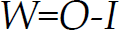
A special case of PN is the multi reentrant flow-line system (MRF), see Figure 1. For MRF systems, we partition the set of places, P = J ∪ R ∪ PI ∪ PO, with the places in J, R, PI, PO representing respectively, the jobs performed, the availability of resources, input of parts, and output of products. Each part path starts with a PI-place and terminates with a PO-place. We denote the set of job places J for part type j as J_j so that J = ∪_j J_j.

Fig. 1.

MRF system

Let the set of transitions along part path j be x_j1, x_j2, …, x_jL_j, with x_j1 and x_jL_j being the initial and terminal transitions respectively.

R(p) is the set of resources needed by job p. For any resource r ∈ R define the jobs performed by r as J(r). We partition the resource set R as R_s and R_ns, with R_s being the set of shared resources, i.e. those needed for more than one job, and R_ns being the set of non-shared resources. Then, |J(r)| = 1 if r ∈ R_ns and | J(r)| > 1 if r ∈ R_s, with |S| denoting the cardinality of a set S (i.e. the number of elements).

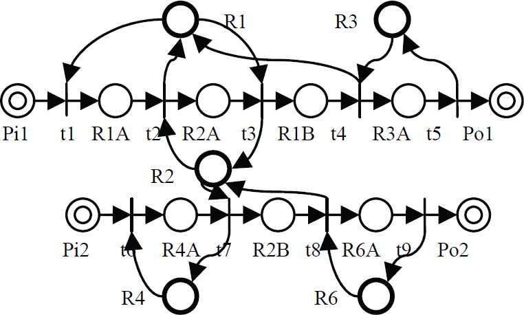
More general than MRF are the free-choice multi reentrant flow-line systems (FMRF), which have no predetermined resource allocation for the jobs. That is, several different resources may be capable and available to perform a specific job. Then, routing decisions may be required along the part path about which resources to use for the next job, see Figure 2.

Fig. 2.

FMRF system

We formally define FMRF systems as a class of systems satisfying the following properties ((/> being the empty set):

Properties of FMRF

p ∈ P, • p ∩ p • = φ

on part path j, x_j1 • ∩ P\J = φ and •x_jLj ∪ P\J = φ

∀p ∈ J, •• p ∩ R = p •• ∩ R = R(p) with |R(p)| = 1

p ∈ J, |p •|≥ 1

∀p_i, p_k ∈ J_j, i ≠ k, p_i ≠ p_k

∀p_i ∈ J_j, p_k ∈ J_l, j ≠ l, p_ji • ∩ p_lk • = φ

R_s ≠ φ

This means that there are: (1) no self loops, (2) each part path has a well-defined beginning and an end, (3) every job requires only one resource with no two consecutive jobs using the same resource, (4) there may be some jobs that can be done by different resources (i.e. routing decisions may have to be made), (5) there are no part path loops, (6) for any two distinct jobs on different part paths there is no assembly, i.e. two part paths cannot merge into one, (7) there are shared resources.

According to property 3, R(p) = •• p ∩ R = p •• ∩ R, with the cardinality |R(p)| = 1; Under the foregoing assumption, one has J(r) = r •• ∩ J = •• r ∩ J.

Property 4 distinguishes MRF from FMRF systems. A FMRF system can have |p •| > 1 for some p ∈ J, so that routing decisions are needed. We call such job places ‘decision places’. In MRF, one has |p• = 1 ∀p ∈ J. That is, MRF are a special class of FMRF. A transition x ∈ p • is said to be a posterior transition of p. A decision place has multiple posterior transitions, i.e. |p •| > 1. The resources used by decision places are called decision resources.

Figure 1 shows a MRF system, while Figure 2 shows a FMRF system. In Figure 1 the part paths are independent and neither split nor recombine. R1 is a shared resource along a single part path, and R2 is a shared resource between two part paths. In Figure 2 the part paths split at decision places. The decision places are B1 and B2, each followed by two transitions. A choice is required there to decide which resource (R1 or R2, respectively R3 or R4) to use for the next job.

C. Circular Wait (CW)

The following background is taken from [Ezpeleta et al. 1995, Lewis et al. 1998, Wysk et al. 1991]. We say resource r_i waits for resource r_j (denoted r_i → r_j) if the availability of r_j is an immediate prerequisite for the release of r_i, i.e., •r_i ∩ r_j • ≠ φ. A wait relation digraph is defined as G_w = (R, A) where R is the set of nodes and A = {a_ij} is the set of edges with a_ij drawn if r_i → r_j (i.e. each a_ij represents a transition in •r_i ∩ r_j •). In G_w, define an R-path between r_i and r_k as a set of R-places such that r_i → r_j→…→r_k. Then r_i is said to wait over an R-path for r_k, denoted r_i → r_k, if there is an R-path between r_i and r_k. A circular wait (CW) is a set of resources C ⊂ R, with |C|>1, such that for any ordered pair ${r_{i}, r_{j}} \subset C, r_{i} \mapsto r_{j}$ . A CW always contains at least one shared resource.

The simplest CW is a set of resources C ⊂ R, such that for some appropriate re-labeling, one has r₁ → r₂ → … → r_q → r₁, with r_i ≠ r_j for i ≠ j, 1 ≤ i, j ≤ q. This will be referred to as a simple circular wait. A simple circular wait is a simple circuit in the graph and is a CW not containing any other CW. Consider a wait relation graph G_w and a CW C ⊂ G_w. Then for every r ∈ C, there exists at least one simple circular wait σ ⊂ C such that r ∈ σ. A CW is a strongly connected sub graph in the digraph G_w and can be obtained by taking unions of non-disjoint simple CW.

Given a CW C = {r_i}, one can partition the set of transitions •r_i as •r_i = •r_io ∪ •r_i+, where •r_io = {x ∈ T | • x ∩ C ≠ φ}, the set of input transitions of r_i with input arcs from some other r_j ∈ C, and •r_i+ = {x ∈ T | •x ∩ C = φ}, the set of input transitions of r_i with no input arcs from any other r_j ∈ C. We loosely say that the transitions •r_io are ‘in the CW C’.

The job set of CW C = {r_i} is given by $J (C) = \cup_{i = 1}^{n} J (r_{i})$ . Partition this as J(C) = J(C)₊ ∪ J(C)₀, where J(C)₀ = {p ∈ J(C) | p • ∈ •r_io,r_i ∈ C} and J(C)₊ = {p ∈ J(C) | p• ∈ •r_i+, r_i ∈ C}.

Note that for FMRF, one may have J(C)₊ ∩ J(C)₀ ≠ φ. In fact, if p ∈ J(C) is a decision place with C a simple CW, i.e. |p • > 1 so that it has more than one posterior transition, then, p ∈ J(C)₊ and p ∈ J(C)₀. This is precisely what distinguishes deadlock avoidance in MRF from deadlock avoidance in FMRF systems.

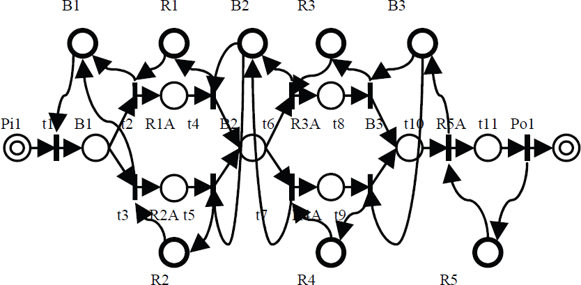
Figure 3 shows a FMRF system. Here, R1-B2-M1-B3 is a CW C. Here, r1a, m1, b2 and b3 are in J(C)0 and r1b is in J(C)+ b2 and b3 are decision places and B2 and B3 are the respective decision resources. In FMRF systems, due to their construction, the decision places (b2 and b3 in this example) are also a part of J(C)₊.

Fig. 3.

FMRF system

D. Marking, Place Vector

A place p ∈ P = J ∪ R ∪ PI ∪ PO is said to be marked when it contains a token, which depending on the place containing it indicates an ongoing job, the existence of an available resource, a part in, or a product out. In a FMRF, the initial marking vector denoted as mo assigns tokens only to R and PI-places. It is assumed that the PO-places are always empty.

Given p ∈ P, m(p) denotes the marking of p, i.e. the number of tokens in p. Given a set of places S, m(S) denotes the number of tokens in S. A set of places is said to be unmarked or empty if none of its places has any tokens.

Given the set of places P, the PN place vector, or p-vector, p has dimension of |P|, and one element corresponding to each place. Let the set of all places be P = {p₁, p₂, …, p_Q}. Then the place vector has Q elements. Any set of m places {p_ik ∈ P|k = 1, 2, …, m} can be represented as a |P|-vector p having m entries ${\vec{p}}_{i_{k}} = 1$ and zero entries otherwise. The PN marking vector $m (\vec{p}) = [m (p_{1}) m (p_{2}) \dots]^{T} \in N^{| P |}$ , with the natural numbers N = {0, 1, 2 …}, gives the number of tokens in each place.

Define the PN transition vector, or x-vector, x to have dimension of |T|, and one element x_i corresponding to each transition. Let the set of all transitions be T = {x₁, x₂, … x_L}. Then the transition vector has L elements. A set of m transitions {x_{i
_k} ∈ T|k = 1, 2, …, m} can be represented as an L-vector x having m entries x_{i
_k} = 1 and zero entries otherwise.

The well-known PN marking transition equation [Peterson 1981],

m^{+} \vec{(p)} = m \vec{(p)} + W^{T} x

(2)

gives the new marking vector $m^{+} (\vec{p}) = m (\vec{p}) + W^{T} x$ in terms of the previous marking vector $m^{+} (\vec{p})$ and the transitions that have fired appearing as 1's in x.

A p-invariant is defined as a set of resources and places that is in the null space of W. i.e.

W p = 0.

(3)

Note that if p is a p-invariant, then

p^{T} m^{+} \vec{(p)} = p^{T} m \vec{(p)} + p^{T} W^{T} x = p^{T} m \vec{(p)}

so that the number of tokens in a p-invariant is constant. One type of p-invariant is given by any resource plus all of its jobs, r ∪ J(r).

E. Circular Blocking

A circular blocking CB is a circular wait that is empty and will always remain so [Lewis et al. 1998, Mireles et al. 2002, Wysk et al. 1991]. That is, for a CW C = {r_i}:

m(C)=0, and

no tokens will ever be added to C.

In this situation, one is said to have deadlock, where the resources in the CW are waiting for each other and will never again become available. If a resource on a given part path is involved in a CB, then all downstream activity along that part path will eventually end. That is, after some time, the downstream jobs on that part path will never again be performed. Let CB = {C_i} be a set of disjoint CW. Then, C is said to be in CB if each CW C_i is in CB.

F. Siphons

The analysis of CB and deadlock can be carried out formally using the notion of siphon. A siphon is a set of places having the property that its input transition set is contained in its output transition set i.e.

∙ S \subset S ∙

(4)

A siphon has the key property that, once it is unmarked, it remains so.

A minimal siphon of a CW C is the smallest siphon containing the CW. Define a critical siphon for a CW C as a smallest siphon which has the property that a CW is a CB if and only if the critical siphon is empty. It is shown in [Lewis et al. 1998, Mireles et al. 2002, Zhou et al. 2005] that a minimal siphon in MRF is a critical siphon.

For MRF systems, for every CW C, the set of places Ŝ_c defined by

{\hat{S}}_{c} = C \cup J (C)_{+}

(5)

is a minimal siphon as well as a critical siphon, where J(C)₊ was defined earlier [Mireles et al. 2002, Wysk et al. 1991].

In the case of FMRF systems, this object is still a minimal siphon, but it cannot be used in deadlock analysis due to decision places. Hence it is not a critical siphon. Following Lemmas are true for FMRF systems [Ballal et al. 2007].

Lemma 1: For FMRF systems, Ŝ_c is a minimal siphon for the CW C.▪

Lemma 2: Let C be a simple CW and Ŝ_c contain a decision place whose associated decision resource is not a shared resource, then Ŝ_c contains a p-invariant and can never be empty.▪

3. Critical Siphons and Critical Subsystems for FMRF

Lemma 1 shows that Ŝ_c given by (5) is indeed a minimal siphon, even for FMRF, but Lemma 2 shows that in some situations for FMRF, Ŝ_c can never be empty. Since deadlock can still occur in such situations, it is necessary to provide an alternative formula for critical siphons for FMRF.

A. FMRF Critical Siphons

Let C_s be the set of all simple CWs in a FMRF system. Let p be a decision place with resource place r_p = R(p). Define the set of all the simple CWs in C_s containing the decision resource r_p as

C_{p} = {C \in C_{s} | r_{p} \in C}

(6)

Given a CW C, let the set of its decision places be

J_{d e c} (C) = {p \in J (C) | | p ∙ | > 1}

(7)

Define,

C_{p} (C) = {C_{p} | p \in J_{d e c} (C)}

(8)

which is the key to deadlock analysis in FMRF systems.

We need to recursively compute Cp(C), as each individual simple CW in C_p(C) defined in (8) may contain more decision resources, and so on as shown in Figure 4. Hence we need an algorithm to calculate C_p(C). Algorithm 1 shows a modified version of the greedy activity selector algorithm [Corman et al. 2001].

Fig. 4.

Tree representation of simple CW dependence through decision places

Algorithm 1:

Compute C_p(C) for a CW C Given a CW C,

Note that this algorithm computes the set C_p(C) for a single CW. The time complexity of this algorithm is known to be linear [Corman et al. 2001] as the running time is directly proportional to |CW_r|. Hence, if R_n is the number of resources in FMRF, the complexity from step 4 to 5 is O(R_n x | CW_r|). The complexity for computing C_p(C) for all the CWs in the system is O((R_n x |CW_r|)²). This set is converted to a single row by using union of all the rows of C_p(C) (Explained in Sections 4 and 5). Also, when this algorithm terminates, C_p(C)=C_p(C_p(C)). This algorithm terminates in one of the two ways:

J(C_p(C))₊ ∩ J(C_p(C))₀ = φ or

J(C_p(C))₊ ∩ J(C_p(C))₀ ≠ φ.

Given a CW C define the object,

S_{c} = C_{p} (C) \cup J (C_{p} (C))_{+}

(9)

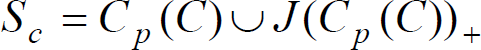
The next results from [Ballal et al. 2007] show that S_c is a critical siphon for C for FMRF systems under a certain condition.

Theorem 1: Given C_p(C) and let J(C_p (C))₊ ∩ J(C_p (C))₀ = φ. Then C_p(C) is in CB if and only if S_c is empty.

Theorem 2: Let J(C_p(C))₊ ∩ J(C_p(C))₀ ≠ φ. Then C_p(C) can never be in CB.

Theorem 3: If J(C_p (C))₊ ∩ J(C_p (C))₀ = φ then CW C is in CB if and only if C_p(C) is in CB.

B. FMRF Critical Subsystems

For better perspective on achieving dispatching policies with deadlock avoidance, the concept of critical subsystems [Lewis et al. 1998] is introduced. To avoid deadlock, work in progress (WIP) must be limited within certain critical subsystems that are constructed by using critical siphons, called MAXWIP.

A critical subsystem for a CW C in MRF is defined as the set of J-places J(C)₀. In case of FMRF, Critical Subsystem for a CW C can be defined if J(C_p(C))₀ ∩ J(C_p(C))₊ = φ and in this case it is defined as the set of J-places J(C_p(C))₀. Define the set S_c* = S_c ∪ J(C_p(C))₀ called the support of the binary p-invariant that minimally covers S_c. Then the following Lemmas are true [Ballal et al. 2007].

Lemma 3: In FMRF, a simple CW C is not in deadlock if and only if one has m(J(C_p(C))₀m(S_c*)▪

The condition m(S_c*) can be given in terms of the initial marking of C_p(C), since for FMRF, the initial marking assigns tokens only to R and PI places.

Note that one can now avoid deadlock of a simple CW C by ensuring that the marking of its critical subsystem S_c* is less than the total marking of the initial resources in C_p(C). To be able to analyze FMRF systems (and for MRF systems) and all its possible deadlock structures, we need to identify the set of all CWs i.e simple CWs and CWs composed of union of non-disjoint simple CWs (unions through shared resources among simple CWs) [Lawley 2000, Lewis et al. 1998]. Let us denote this set as CW_r. Lemma 4: In FMRF, there is no CB in the system if and only if for every C ∈ CW_r, one has m(J(C_p(C))₀ less than the initial marking of C_p(C).▪

These results show that we can avoid deadlock by MAXWIP, i.e. limiting WIP in all the critical subsystems.

4. Matrix Formulation for FMRF

PN provides great pictorial insight and mathematical techniques for analysis, but they have sometimes had the deficiency of not providing an efficient computational framework for simple computer-based analysis. A matrix framework for computing structural objects of a PN can correct these deficiencies [Lewis et al. 1998]. Note that the matrix formulation for PN objects is not the main contribution of this paper. Our main contribution resides in the matrix formulation of deadlock avoidance in FMRF systems.

Commensurate with the partitioning P = J ∪ R ∪ PI ∪ PO with J, R, PI, and PO being the sets of job places, resource places, input places, and output places respectively, partition the place vector as

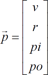
\vec{p} = [\begin{matrix} ν \\ r \\ p i \\ p o \end{matrix}]

with v ∈ J, r ∈ R, pi ∈ PI, po ∈ PO.

Similarly, partition the input incidence matrix as I = [F_v F_r F_i F_o]. Note that there are no input arcs to transitions from the places in PO, so that F_o = 0, a matrix of zeros. Partition the output incidence matrix as O = [S_v^T S_r^T S_i^T S_o^T]. Note that there are no output arcs from transitions to the places in PI, so that S_i=0. These sub-matrices are Boolean matrices having entries of 0 or 1.

Given Boolean matrices A = [a_ij] and B = [b_ij], define a logical or/and matrix algebra wherein addition operations are replaced by logical ‘or’ and multiplication operations by logical ‘and’. That is, the matrix product is defined by C = A ⊗ B with

c_{i j} = (a_{i 1} \land b_{1 j}) \lor (a_{i 2} \land b_{2 j}) \lor (a_{i 3} \land b_{3 j}) \lor \dots

with ∧ denoting logical ‘and’ and ∨ denoting logical ‘or’. The matrix sum is defined by C = A ⊕ B with

c_{i j} = a_{i j} \lor b_{i j} .

Note that these matrix products are easily performed using standard software programs including MATLAB^®, etc.

Then one has computational methods for computing PN objects based on the following results [Ballal et al. 2007].

Let v represent a set of job places. Then

v • is represented by the vector F_v ⊗ v

• v is represented by the vector S_v^T ⊗ v

Let r represent a set of resource places. Then

r • is represented by the vector F_r ⊗ r

•r is represented by the vector

Let x represent a set of transitions. Then

x• ∩ J is represented by the vector S_v ⊗ x

x• ∩ R is represented by the vector S_r ⊗ x

•x ∩ J is represented by the vector F_v^T ⊗ x

•x ∩ R is represented by the vector F_r^T ⊗ x

A. Circular Waits in Matrix Form

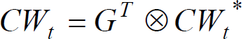
A wait relation digraph in FMRF is defined as [Mireles et al. 2002],

W = [\begin{matrix} O_{r} & S_{r} \\ F_{r} & O_{t} \end{matrix}]

(10)

where O_r is a zero-matrix having nxn elements, O_t is a zero-matrix having mxm elements, n be the number of resources or rows (column) of S_r (F), and m be the number of transitions or rows (columns) of F (S_r). This is a digraph of transitions T and resources R.

For example, this digraph can be obtained by erasing all the jobs places from Figure 3, and keeping the resources, the transitions, and all the links between them, as shown in Figure 5.

Fig. 5.

Graphical representation of digraph matrix W

Note that, using this digraph matrix W with the binary string algebra algorithm given in [Mreles et al. 2002, Zhou et al. 2005], we get the set C_w = [CW_r* CW_t*], where CW_r* is the set of simple CW of resources and CW_t* is a set of simple CW of transitions.

In order to find the complete set of simple CWs and the union of non-disjoint simple CWs, we use the Gurel algorithm [Lewis et al. 1998] which gives a matrix G. G provides the set of composed CWs (rows) from unions of simple CWs (columns) i.e. an entry of ‘1’ in every (i, j) position implies j^th simple CW is included in the i^th composed CW. Then, we can calculate the set of loop resources CW_r and loop transitions CW_t using the following constructions,

C W_{r} = G^{T} \otimes {C W}_{r}^{*}

(11)

C W_{t} = G^{T} \otimes {C W}_{t}^{*}

(12)

Note that * denotes a simple CW, while CW_r and CW_t refer to all the CWs (i.e. simple and their unions).

B. Matrix Algorithm for Computing Cp(C)

Property 4 of FMRF, i.e p ∈ J, |p• ≥ 1, is what differentiates FMRF from MRF systems. We apply this property of FMRF to compute C_p(C) using matrices. To do so, we must first compute C_p and J_dec(C) for each CW as required to run Algorithm 1. The next algorithm shows a routine which can easily be implemented using tools such as MATLAB^®, to compute C_p and J_dec(C).

Algorithm 2:

Calculating C_p using matrices

After computing C_p, J_dec(C) and the initial C_p(C) using Algorithm 2, we use Algorithm 1 to compute C_p(C) recursively. Note that Algorithm 1 only computes the set C_p(C) for a CW C under consideration. Then, this set is converted to a single row by using union of all the rows of C_p(C). The same procedure is followed for all the other CWs in the system using a simple ‘for loop’ to get the complete set C_p(C) for all the CWs in the system.

The complexity of Algorithm 2 is O(|(CW_r)|) as the running time is directly proportional to the number of CWs in the system. For calculating the same for all the CWs in the system, the complexity is O(|(CW_r)|²).

C. Critical Siphons/Critical Subsystems In Matrix Form

In this section we use matrices to compute the PN objects i.e. Critical Siphons and Critical Subsystems required in Section 3 for deadlock analysis in FMRF systems.

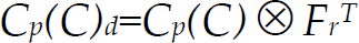
•C and C• are the set of input and output transitions from a CW C. Once CW_r is constructed, we use Algorithm 2 and then Algorithm 1 to construct C_p(C) for each C ∈ CW_r. Let •C_p(C) and C_p(C)• be the set of input and output transitions from C_p(C). In matrix formulation, it is denoted as _dC_p(C) and C_p(C)_d respectively. It is computed as:

_{d} C_{p} (C) = C_{p} (C) \otimes S_{r}

(13)

C_{p} (C)_{d} = C_{p} (C) \otimes F_{r^{T}}

(14)

To find the set of transitions CW_t(C_p(C)) between resources in the set C_p(C), we use,

C W_{t} (C_{p} (C)) =_{d} C_{p} (C) \otimes C_{p} (C)_{d}

(15)

The critical subsystems J(C_p(C))₀ for a given CW_r are given by,

J (C_{p} (C))_{0} = C W_{t} (C_{p} (C)) \otimes F_{ν}

(16)

The siphon job sets J(C_p(C))₊ are given by,

J (C_{p} (C))_{+} =_{d} C_{p} (C) \otimes \bar{(_{d} C_{p} (C) \otimes C_{p} (C)_{d})} \otimes F_{ν}

(17)

Now we have all the formulations to compute using matrices the objects required for deadlock avoidance using Theorem 3 and Lemma 4.

D. MAXWIP Dispatching Policy For Deadlock Avoidance In FMRF

Lemma 4 formulates the MAXWIP dispatching policy for deadlock avoidance in FMRF systems. According to this policy, CB in FMRF is avoided by limiting WIP in the critical subsystems of each CW C. This policy can be implemented as a real-time deadlock avoidance control scheme by controlling the firing of the precedence transitions of the critical subsystems.

5. Implementation Results

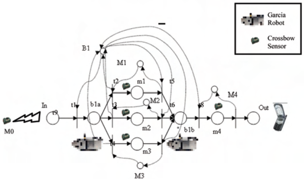
To show the effectiveness of the proposed strategy, an application scenario is discussed in this Section. A warehouse monitoring system is implemented at Automation and Robotics Research Institute (ARRI). The test-bed consists of an Acroname^® Garcia robot which acts as a mobile resource while five Crossbow^® Mica2 sensors act as stationary resources. The mobile robots are also endowed with Crossbow^® sensors, so that we have a test-bed consisting of mobile and stationary sensors. Also, MIT cricket sensors (ultrasound ranging) are used for localization of the mobile resources. All the resources can communicate with each other for transmisson of data to and from the base-station. Suppose the rule-base for this application is given as shown in Table 1.

Table 1.
Rule-Base for Mission in FMRF

Mission 1 Intruder detected by Sensor M0.

Task no. Tasks to be done

Task 1 – b1a Garcia Robot (B1) goes to sensor M0 to verify data

Task 2, 3, 4 – m1, m2, m3 (Routing jobs) Sensors M1, M2, M3 take sensor readings and send it to Garcia Robot (B1)

Task 5 – b1b Garcia Robot (B1) goes to sensor M4 for relaying all the information

Task 6 - m4 Sensor M4 relays information to base-station

Output Base-station makes decision and alerts the authorities

Figure 6 shows the Petri Net description of the rule-base described in Table 1.

Fig. 6.

Petri Net for the Mission in Table 1

When the number of tasks and resources are increased, the formulation of the required system matrices becomes cumbersome. The LabVIEW^® toolkit developed at ARRI generates the matrices with a default conflict resolution matrix automatically when the resources are assigned to the tasks. The user can either manually change the resource allocation or the resource allocation can be changed automatically. Figure 7 shows the front panel of the toolkit. The toolkit also generates the Petri Net for better visualization.

Fig. 7.

LabVIEW toolkit for PN and Matrices generation

We implement the same mission first without the deadlock avoidance algorithm. Here, we find that,

\begin{aligned} C W_{r} = & \begin{matrix} \begin{matrix} B 1 M 1 M 2 M 3 M 4 \end{matrix} \\ [\begin{matrix} 1 & 1 & 0 & 0 & 0 \\ 1 & 0 & 1 & 0 & 0 \\ 1 & 0 & 0 & 1 & 0 \\ 1 & 1 & 1 & 0 & 0 \\ 1 & 1 & 0 & 1 & 0 \\ 1 & 0 & 1 & 1 & 0 \\ 1 & 1 & 1 & 1 & 0 \end{matrix}] \end{matrix} C_{p} (C) = \begin{matrix} \begin{matrix} B 1 M 1 M 2 M 3 M 4 \end{matrix} \\ [\begin{matrix} 1 & 1 & 1 & 1 & 0 \\ 1 & 1 & 1 & 1 & 0 \\ 1 & 1 & 1 & 1 & 0 \\ 1 & 1 & 1 & 1 & 0 \\ 1 & 1 & 1 & 1 & 0 \\ 1 & 1 & 1 & 1 & 0 \\ 1 & 1 & 1 & 1 & 0 \end{matrix}] \end{matrix} \\ J (C_{p} (C))_{+} = \begin{matrix} \begin{matrix} b 1 a m 1 m 2 m 3 b 1 b m 4 \end{matrix} \\ [\begin{matrix} 0 & 0 & 0 & 0 & 1 & 0 \\ 0 & 0 & 0 & 0 & 1 & 0 \\ 0 & 0 & 0 & 0 & 1 & 0 \\ 0 & 0 & 0 & 0 & 1 & 0 \\ 0 & 0 & 0 & 0 & 1 & 0 \\ 0 & 0 & 0 & 0 & 1 & 0 \\ 0 & 0 & 0 & 0 & 1 & 0 \end{matrix}] \end{matrix} \\ J (C_{p} (C))_{0} = \begin{matrix} \begin{matrix} b 1 a m 1 m 2 m 3 b 1 b m 4 \end{matrix} \\ [\begin{matrix} 1 & 1 & 1 & 1 & 0 & 0 \\ 1 & 1 & 1 & 1 & 0 & 0 \\ 1 & 1 & 1 & 1 & 0 & 0 \\ 1 & 1 & 1 & 1 & 0 & 0 \\ 1 & 1 & 1 & 1 & 0 & 0 \\ 1 & 1 & 1 & 1 & 0 & 0 \\ 1 & 1 & 1 & 1 & 0 & 0 \end{matrix}] \end{matrix} \end{aligned}

Here we see that J(C_p(C))₊ ∩ J(C_p(C))₀ = φ. Hence, when tokens are in the tasks b1a, m1, m2 and m3 at the same time, deadlock will occur as they form the critical subsystem. Hence, when the mission is triggered for the second time, as long as tasks m1, m2 and m3 are in progress and the token is in b1a, deadlock will occur, as shown in the implementation event trace timing diagram in Figure 8. The event trace timing diagram provides a good illustration of occurance of deadlocks in complicated systems and their avoidance e.g. see ([Giordano et al. 2206 and Mireles et al. 2002]).

Fig. 8.

Implementation without Deadlock Avoidance

We see that the resources B1, M1, M2 and M3 are never released and hence the tasks b1b and m4 are never completed. The MAXWIP dispatching policy formulated for deadlock avoidance in FMRF systems avoids this deadlock by limiting the work in progress (WIP) in the critical subsystems of each CW. According to this policy, as long as the tasks m1, m2 and m3 are in progess, the task b1b is not allowed to start. Once the tasks m1, m2, and m3 are completed, the task b1b is allowed to start and deadlock is successfully avoided. The event trace timing diagram is shown in Figure 9.

Fig. 9.

Implementation with Deadlock Avoidance

From the Figure we can see that there is no deadlock in the system and all the tasks are performed correctly.

6. Conclusions

Presence of shared resources and decision resources in a mobile wireless sensor network can create deadlocks. Such systems can be modeled as a FMRF system. A theory for deadlock avoidance in FMRF is provided in this paper. It is shown that the occurrence of decision places, which are followed by two or more resource paths, means that the usual notion of critical siphon used in MRF does not apply for FMRF. Therefore, we define a new notion of critical siphon for FMRF that is tied to deadlock avoidance. A MAXWIP dispatching policy is formulated for deadlock avoidance in FMRF systems. According to this policy, it has been shown that the work in progress (WIP) must be limited in the critical subsystems to avoid deadlock. A matrix formulation that efficiently computes the various PN objects required for deadlock avoidance in FMRF has been provided. This matrix formulation allows fast and efficient numerical computation techniques to be applied to PN analysis. An implementation which shows the efficiency of the proposed deadlock avoidance policy in Mobile WSN is provided. Note that this formulation is applicable to only first order deadlocks. There are other deadlock structures called second order deadlocks which occur due to the presence of key resources. Deadlock avoidance in FMRF in presence of key resources is part of our future work.

Footnotes

7.

This research was supported ARO grant DAAD 19-02-1-0366; ARO grant ARO W91NF-05-1-0314; NSF grant IIS-0326505; NSF grant CNS-0421282, DOE/SBIR grant 26-3903-81, NI Lead User grant, Texas ARP grant 14-748779.

References

Ballal

Lewis

Mireles

Sreenath

(2007), “Deadlock avoidance for free choice multi-reentrant flow lines: Critical siphons and critical subsystems”, Proc. Mediterranean Conf. Control & Automation, Athens, Greece, June 2007

Ballal

Giordano

Lewis

(2006), “Deadlock Free Dynamic Resource Assignment in Multi-Robot Systems with Multiple Missions: A Matrix-Based Approach,” Proceedings of Mediterranean Conference on Control & Automation, Ancona, Italy, June 2006.

Butler

Rus

(2003), “Event-based motion control for mobile-sensor network”, IEEE Transactions on Pervasive Computing, vol.2 issue 4, October-December 2003

Cortes

Martinez

Karatas

Bullo

(2004), “Coverage control for mobile sensing network”, IEEE Transactions on Robotics and Automation, Vol. 20, Issue 2, pp. 243–255, April 2004

Chong

Kumar

(2003), “Sensor Networks: Evolution, Opportunities and Challenges”, Proceedings of the IEEE, col. 91, no.8, August 2003

Corman

Leisenson

, and Rivest

(2001), Introduction to Algorithms, Prentice Hall of India, 2001.

Dantu

Rahimi

Shah

Babel

Dhariwal

Sukhatme

(2005), “Robomote: enabling mobility in sensor networks”, Information Processing in Sensor Networks, 2005. IPSN 2005. Fourth International Symposium on 15 April 2005 Page(s):404–409

Ezpeleta

Colom

J.M.

Martinez

(1995); “A Petri net based deadlock prevention policy for flexible manufacturing systems”, IEEE Transaction on Robotics and Automation, Volume 11, Issue 2, April 1995 Page(s):173–184

Ezpeleta

Recalde

(2002), “A deadlock avoidance approach for nonsequential resource allocation systems,” in Proc. IEEE Int Conf. Syst., Man, Cybern., Oct. 2002.

10.

Fanti

M. P.

Maione

and Turchiano

(2001), “Distributed Event-Control for Deadlock Avoidance in Automated Manufacturing Systems,” International Journal of Production Research 39(9), 2001, Page(s): 1993–2021.

11.

Fanti

M.P.

Maione

Turchiano

(2000); Comparing digraph and Petri net approaches to deadlock avoidance in FMS IEEE Transactions on Systems, Man and Cybernetics, Part B, Volume 30, Issue 5, Oct. 2000 Page(s):783–798

12.

Fanti

Zhou

(2004), “Deadlock control methods in automated manufacturing systems,” IEEE Transactions on Systems, Man, and Cybernetics - Part A: Systems and Humans, 34(1):5–22, 2004.

13.

Gerkey

Mataric

(2002), “Sold! Auction methods for multirobot coordination”, IEEE Transactions on Robotics and Autoation, vol. 18, no. 5, October 2002

14.

Gerkey

Mataric

(2004), “A formal analysis and taxonomy of task allocation in multi-robot systems”, Int. Journal of Robotics Research, vol.:18, no.5, September 2004

15.

Giordano

Ballal

Lewis

Turchiano

Zhang

J. B.

(2006), “Supervisory Control of Mobile Sensor Networks: Math Formulation, Simulation, Implementation,” IEEE Transactions on Systems, Man and Cybernetics, Part B, Volume 36, Issue 4, Aug. 2006 Page(s):806–819.

16.

Giordano

Lewis

Mireles

(2005), Turchiano

, “Coordination control policy for mobile sensor networks with shared heterogeneous resources”, Proceedings of the IEEE International Conference on Control and Automation, Budapest, June 2005

17.

Giordano

Lewis

Turchaino

Ballal

Yeshala

(2005), “Matrix Computational Framework for Discrete Event Control of Wireless Sensor Networks with Some Mobile Agents,” Proceedings of the Mediterranean Conference on Control & Automation, Limassol, Cyprus, June 2005.

18.

Gurel

Bogdan

Lewis

(2000), “Matrix approach to deadlock-free dispatching in multi-class finite buffer flowlines”, IEEE Transactions on Automatic Control, Vol. 45, Issue 11, November 2000, pp.2086–2090

19.

Judd

Zhang

Deering

Lipset

, “A Scalable Deadlock Avoidance Algorithm for Flexible Manufacturing Systems with Free Choice in Part Routing,” Proceedings of IEEE American Control Conference, 2000.

20.

Lawley

(2000) “Integrating Routing Flexibility and Algebraic Deadlock Avoidance Policies in Automated Manufacturing Systems,” International Journal of Production Research, 2000, Page(s): 2931–2950.

21.

Lewis

Gurel

Bogdan

Docanalp

Pastravanu

(1998), “Analysis of deadlock and circular waits using a matrix model for flexible manufacturing systems”, Automatica, vol.34, no. 9, September 1998

22.

Lewis

(2004), “Wireless sensor networks,” Smart environments: Technologies, Protocols, and Applications, ed. Cook

D. J.

and Das

S. K.

, John Wiley, New York, 2004.

23.

Maione

Naso

(2001), “Modeling Evolutionary Supervisors for Multi-Agent Manufacturing Control with Discrete Event Formalism,” Proceedings of IEEE Mountain Workshop on Soft Computing in Industrial Applications SMCia/01, June 2001.

24.

Mireles

Lewis

Gurel

(2002), “Implementation of a deadlock avoidance policy for multipart reentrant flow lines using a matrix-based discrete event controller”, Proceedings of the International symposium on advances in robot dynamics and control, New Orleans, November 2002

25.

Murata

(1989), “Petri Nets: Properties, Analysis and Applications.” Proceedings of the IEEE, vol.77, no.4, April 1989, pp.541–80

26.

Ozmutlu

And Harmonosky

C.M.

(2005), “A Real Time Methodology for Minimizing Mean Flowtime in FMSs With Routing Flexibility: Threshold Based Alternate Routing,” European Journal of Operational Research, 2005, Pages(s): 369–384.

27.

Peterson

J. L.

(1981), “Petri Net Theory and the Modeling of Systems,” Prentice-Hall, Englewood Cliffs, NJ, 1981.

28.

Piroddi

Ferrarini

(2005), “A Modular Approach for Deadlock Avoidance in FMS,” Proceedings of IEEE Conference on Decision and Control, 2005.

29.

Puccinelli

Haenggi

(2005), “Wireless Sensor Networks: Applications and Challenges of Ubiquitous Sensing”, IEEE Circuits and Systems Magazine, vol. 5, pp. 19–29, August 2005.

30.

Reveliotis

(2001), “On the Siphon-based Characterization of Liveness in Sequential Resource Allocation Systems,” Tech. Report, School of Industrial & Systems, Eng. Georgia Tech, 2001.

31.

Sinopoli

Sharp

Schenato

Schaffert

Sastry

(2003), “Distributed Control Applications Within Sensor Networks”, Proceedings of the IEEE, vol. 91, no.8, August 2003

32.

Tacconi

Lewis

(1997), “A new matrix model for discrete event systems: application to simulation”, IEEE Control System Magazine, vol.17 October 1997

33.

Wysk

R.A.

Yang

N.S.

Joshi

(1991); “Detection of deadlocks in flexible manufacturing cells”, IEEE Transactions on Robotics and Automation, vol.:7, Issue: 6, December 1991

34.

Xing

K.Y.

B.S.

Chen

H.X.

(1991), “Deadlock Avoidance Policy for Petri-net Modeling of Flexible Manufacturing Systems With Shared Resources,” IEEE Transactions on Automatic Control, Volume 41, Feb 1991 Page(s): 289–295.

35.

Xing

Jin

Feng

(2005), “Deadlock Avoidance Petri Net Controller for Manufacturing Systems with Multiple Resource Service,” Proceedings of IEEE Conference on Robotics and Automation, 2005.

36.

Zhou

M.C.

Fanti

M. P.

(2005), Eds., “Deadlock Resolution in Computer-Integrated Systems,” New York: Marcel Dekker, 2005.

Mission 1	Intruder detected by Sensor M0.
Task no.	Tasks to be done
Task 1 – b1a	Garcia Robot (B1) goes to sensor M0 to verify data
Task 2, 3, 4 – m1, m2, m3 (Routing jobs)	Sensors M1, M2, M3 take sensor readings and send it to Garcia Robot (B1)
Task 5 – b1b	Garcia Robot (B1) goes to sensor M4 for relaying all the information
Task 6 - m4	Sensor M4 relays information to base-station
Output	Base-station makes decision and alerts the authorities

Deadlock Avoidance Policy in Mobile Wireless Sensor Networks with Free Choice Resource Routing

Abstract

Keywords

1. Introduction

2. Petri Net Analysis

A. Petri Nets

F. Siphons

A. FMRF Critical Siphons

4. Matrix Formulation for FMRF

A. Circular Waits in Matrix Form

5. Implementation Results

Footnotes

7.

References