Car-Like Mobile Robot Oriented Positioning by Fuzzy Controllers

Abstract

In this paper, fuzzy logic controllers (FLC) are used to implement an efficient and accurate positioning of an autonomous car-like mobile robot, respecting final orientation. To accomplish this task, called “Oriented Positioning”, two FLC have been developed: robot positioning controller (RPC) and robot following controller (RFC). Computer simulation results illustrate the effectiveness of the proposed technique. Finally, real-time experiments have been made on an autonomous car-like mobile robot called “Robucar”, developed to perform people transportation. Obtained results from experiments demonstrate the effectiveness of the proposed control strategy.

1. Introduction

Human respectful way of transportation is one of the most treated projects in robotic research throughout the world. This new ways of transportation is usually based on electrical car-like mobile robots. Nevertheless, developing fully autonomous electrical car able to move in dynamic outdoor environments is not a trivial task. One of the most crucial problems is to develop an efficient and accurate algorithm allowing the car movement in an unknown environment, while respecting nonholonomic constraints. A part of this problem is to compute in real-time the inputs which imply to reach a desired destination (goal) from any initial location.

Goals are usually expressed in a 2D space by means of two coordinates plus an orientation, [x_G, y_G, θ_G]. This is called an Oriented Goal. Most indoor robots are holonomic and usually have decoupled translation and rotation motion, thus once the 2D position has been attained, final orientation-angle can be easily reached by means of a single rotation. Unfortunately, it is not the case with nonholonomic robots where rotation is coupled to translation. In this case, positioning such robots requires a much powerful and intelligent control strategy. An accurate final orientation is generally needed in outdoor navigation for applications such as people transportation or on autonomous agriculture cars.

Many studies about autonomous navigation applied to nonholonomic robots focused on the design of a global analytic trajectory, composed of straight segments connected with either tangential circular or symmetric clothoîd arcs (Scheuer & Fraichard, 1996). This approaches involves two steps: first planning a feasible trajectory and second designing a control algorithm to follow this trajectory (Manikonda, Hendler & Krishnaprasad 1995; Paromtchik, Garnier & Laugier, 1997). This method has as drawback the lack of reactivity. For more reactive navigation, kinematic constraints have been introduced in the spatial representation (Santos-Victor, Minguez & Montano, 2002).

Instead of following a precise and complete trajectory, other approaches use algorithms which are based on fuzzy sets to drive the robot from an initial position to a goal (Gasós, García-Alegre & García, 1991; Fraichard & Garnier, 2001; Li, Chang & Chen, 2005). All these works has applied their approaches on nonholonomic mobile robots. Authors in (Cuesta, Gomes-Bravo & Ollero, 2004) propose a fuzzy explicit path tracking method, where a fuzzy rule based system is developed to track a pre-computed path for a holonomic small-size robot moving on complex sharp paths.

Nonholonomic vehicles have a complex and non-linear kinematic and dynamics, and therefore the interaction between wheels and ground is extremely difficult to model (Lindgren, Hague, Probert Smith & Marchant, 2002). Fuzzy controllers cope well with the incomplete and uncertain knowledge inherent to the subsystem interactions and non-linearity. In addition, fuzzy controllers are specially suited to embed the human knowledge on an autonomous mobile robot, without using a complete analytical model.

Taking into account the properties of the fuzzy systems, a fuzzy rule based controller has been designed and demonstrated to perform oriented goal navigation in an outdoor natural environment with a commercial lawnmower automated (Garcia-Perez, Garcia-Alegre, Ribeiro & Guinea, 2003). The fuzzy rules encapsulate the expert knowledge in a minimum set, extracted from the observation of the manual operation of an expert driver in a set of field experiments. Inspired from last cited works, we propose in this work a new method based on FLC, to perform an “Oriented Positioning” on an autonomous car-like robot called Robucar.

This paper is organized as follow: Section 2 is started by an introduction to the kinematic model of the Robucar, then “Simple Positioning”, and “Oriented Positioning” principals are exposed. This section ends with computer simulation results of the proposed strategy for simple positioning task. Section 3 is devoted to present real-time experimental results of oriented positioning task applied on the Robucar. It starts with a presentation of simulation results, which are compared and the end to real-time results.

2. Autonomous positioning

The experimental platform used in this work is a car-like mobile robot. Such robot is a mobile vehicle where the front wheels can turn on the left or right, but kept always parallel. The rear wheels are fixed parallel to the car body. Such wheeled robots are systems with hard nonholonomic constraints where differential expressions involving velocity and state vectors are non-integrable. Each wheel presents kinematic constraints due to non-sleeping and non-tilting conditions (Cuesta, Gomes-Bravo & Ollero, 2004). Fig.1 shows a car-like robot with corresponding parameters: [x y] are the rear point R coordinates, and θ is the robot's heading. Linear velocity of the point R is represented by v. The orientation of the front wheels is noted φ, and l is the distance between the rear and the front wheels axes.

Fig. 1.

Car-like mobile robot.

The kinematic equation of the robot is described by:

$$\begin{array}{rl}\stackrel{\bullet }{x}=& \nu \cos \theta \cos \varphi \\ \stackrel{\bullet }{y}=& \nu \sin \theta \cos \varphi \end{array}$$

(1)

$${\begin{array}{c}\theta \end{array}}^{\bullet }=\nu \frac{\sin \varphi }{l}$$

(2)

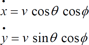
The vector [x y θ]^T is called configuration vector, and the vector [v(t) φ(t)]^T is the control vector. This work is divided into two steps. The first step consists on the implementation of a simple positioning. This task is done by a FLC which makes the robot moving from any initial position to a final destination, respecting nonholonomic constraints. The second task is the oriented positioning.

2.1 Simple Positioning

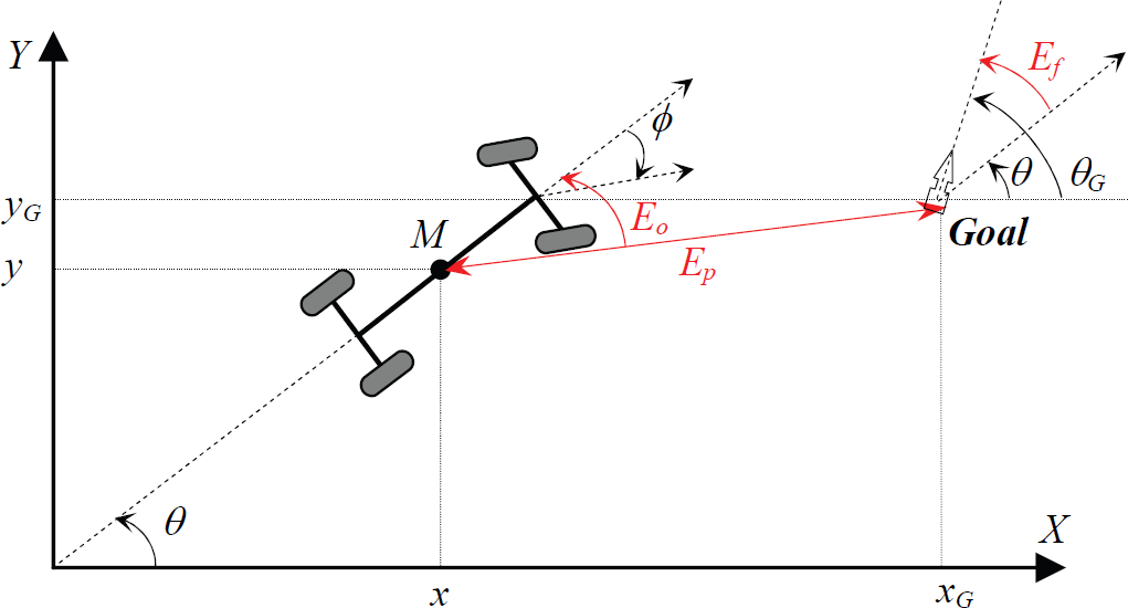
To accomplish a simple positioning of a car-like mobile robot, the control vector [v(t) φ(t)]^T must be computed in real-time, to make the robot moving from its initial position [x_i y_i] to any desired goal [x_G y_G], respecting its nonholonomic constraints. For that, a FLC called “Robot Positioning Controller” (RPC) has been implemented in order to insure the convergence of the robot to the desired goal. The variables used by the RPC are represented on Fig. 2:

Fig. 2.

Simple positioning task.

From this figure:

$$E_p=\sqrt{\mathrm{\Delta }{x}^2+\mathrm{\Delta }{y}^2}$$

(3)

$$E_o=\theta -\mathrm{\Delta }\theta$$

(4)

$$\mathrm{\Delta }\mathrm{x}=\mathrm{x}\mathrm{G}-\mathrm{x}$$

(5)

$$\mathrm{\Delta }\mathrm{y}=\mathrm{y}\mathrm{G}-\mathrm{y}$$

(6)

$$\mathrm{\Delta }\theta =\text{Artan}(\mathrm{\Delta }\mathrm{y},\mathrm{\Delta }\mathrm{x})$$

(7)

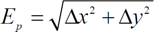
where [x y θ]^T is the configuration vector of the robot with respect to the point M, the middle of its axis. [x_G y_G]^T are the coordinates of the goal (desired position). E_p is called the “Position Error” and E_o is the “Orientation Error”. The implemented RPC has as inputs the two variables E_p and E_o. It provides as output the control vector of the robot [v(t) φ(t)]^T. For the design of the RPC, membership functions are taken triangular.

In Fig. 3(a), the input variable E_p is expressed in meter whereas E_o is expressed in degree in Fig. 3(b). The input variable E_p and the output variable v are decomposed into five fuzzy partitions with triangular membership functions. The same type of membership functions is used for the input variable E_o and the output variable φ, but these two variables have been decomposed into seven fuzzy partitions, in order to make the control more accurate (Fig3(c) and Fig3(d)).

Fig. 3.

(a) Membership functions of the input variable E _p . (b) Membership functions of the input variable E _o . (c) Membership functions of the output variable v. (d) Membership functions of the output variable φ.

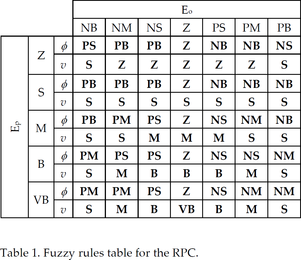
The fuzzy linguistic variables employed to express the membership functions are denoted: Z for “Zero”, S for “Small”, M for “Medium”, B for “Big”, VB for “Very Big”, NB for “Negative Big”, NM for “Negative Medium”, NS for “Negative Small”, PS for “Positive Small”, PM for “Positive Medium”, PB for “Positive Big”. Setting the values for linguistic variables is not a trivial task in the design of a good and efficient FLC. These values have been set after several tests, and taking into account both dynamic characteristics of the robot and user experiences. The fuzzy reasoning rules used for the design of the RPC are summarized in Table 1.

Table 1.

Fuzzy rules table for the RPC.

			Eo
			NB	NM	NS	Z	PS	PM	PB
Ep	Z	φ	PS	PB	PB	Z	NB	NB	NS
		v	S	Z	Z	Z	Z	Z	S
	S	φ	PB	PB	PB	Z	NB	NB	NB
		v	S	S	S	S	S	S	S
	M	φ	PB	PM	PS	Z	NS	NM	NB
		v	S	S	M	M	M	S	S
	B	φ	PM	PS	PS	Z	NS	NS	NM
		v	S	M	B	B	B	M	S
	VB	φ	PM	PM	PS	Z	NS	NM	NM
		v	S	M	B	VB	B	M	S

2.2 Oriented Positioning

Oriented positioning task consists on the accomplishment of a robot positioning, with a desired final orientation. In theory, to accomplish this task, the control vector [v(t) φ(t)]^T can be computed in real-time by a FLC, in order to make the robot moving from any initial configuration [x_i y_i θ_i]^T to any final desired configuration [x_G y_G θ_G]^T, respecting the nonholonomic constraints, as it has been done for simple positioning. Fig. 4 shows the used variables in this case:

Fig. 4.

Oriented positioning task.

The variables E_p and E_o are those used for the case of simple positioning. E_f is computed as follow:

$$E_f={\theta }_G-\theta$$

(8)

E_f expresses the “Final Orientation Error”.

To achieve an oriented positioning task by using one FLC, three input variables are necessary, which are E_p, E_o and E_f. Unfortunately, only two outputs variables (v and φ) are available. The two input variables E_o and E_f are hardly coupled, and can not be controlled in the same time by only the two variables of the robot's control vector. To overcome this problem, we propose to use two FLC in the same time, as it is exposed in the next section.

- Virtual Following:

The proposed solution is the use of a second FLC, called Robot Following Controller (RFC) combined to the first one (RPC used in section 2.1). Indeed, oriented positioning task is divided into two subtasks: the first task is “Simple Positioning” (SP), where the second is “Virtual Following” (VF). Each subtask is performed by one FLC. For the SP, the controller is used to make the robot approaching the desired goal by moving from the initial position [x_i y_i] to an intermediary goal [x_S y_S], called “Sub-goal”, as it is shown in Fig.5. The RPC developed in section 2.1 is suitable for this sub-task. The Sub-goal is chosen near to the final goal [x_G y_G], and can be computed easily offline by geometrical formulas.

Fig. 5.

Virtual Following strategy.

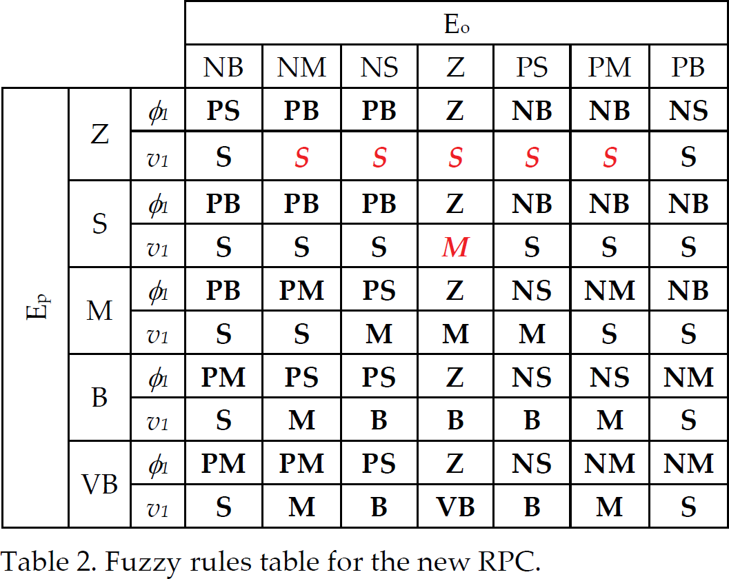
In order to keep velocity variation continuous while performing oriented positioning, the RPC used for the first step must keep the robot moving either if the sub-goal is reached. For that, fuzzy rules table has been modified, especially robot's velocity linguistic variables, as it is shown on Table. 2. The modified variables are in red italic font.

Table 2.

Fuzzy rules table for the new RPC.

			Eo
			NB	NM	NS	Z	PS	PM	PB
Ep	Z	φ 1	PS	PB	PB	Z	NB	NB	NS
		v 1	S	S	S	S	S	S	S
	S	φ 1	PB	PB	PB	Z	NB	NB	NB
		v 1	S	S	S	M	S	S	S
	M	φ 1	PB	PM	PS	Z	NS	NM	NB
		v 1	S	S	M	M	M	S	S
	B	φ 1	PM	PS	PS	Z	NS	NS	NM
		v 1	S	M	B	B	B	M	S
	VB	φ 1	PM	PM	PS	Z	NS	NM	NM
		v 1	S	M	B	VB	B	M	S

Once the robot positioned on the Sub-goal, the second FLC (RFC) has to make the robot moving on a circular trajectory by following a virtual mobile robot. The virtual robot is initially positioned on the Sub-goal. It starts moving when the real robot reaches the sub-goal, and stops on the desired goal by following a circular trajectory. This trajectory is computed to insure that the virtual robot reaches the goal with the desired orientation θ_G, as it is shown in Fig. 5. If the RFC can make the real robot following the virtual robot correctly, we are sure that at the end, the real robot will also reach the goal with the desired orientation θ_G.

The RFC used for the second sub-task has as inputs two variables: E_vp which is the distance between the point M (robot's center) and point V (center of virtual robot), and E_vo which is the angle between the segment MV and the axis of the real robot.

This controller, which is used to make the robot following the virtual robot, has been designed differently from the first one. Dynamic performances are needed to insure a good following and an accurate convergence to the desired goal. The control of velocity must be powerful to keep the robot near to the virtual robot. For that, membership functions of the input variables for the RFC has been set as it is shown in Fig. 6:

Fig. 6.

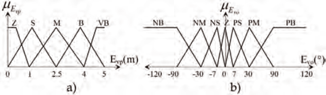
(a) Membership functions of E_vp (b) Membership functions of E_vo.

For the output variables v₂ and φ₂, the membership functions are the same as for the RPC. But the rules table has been changed to make virtual robot's following more accurate. Many linguistic variables (red font size) of the rules table have been changed as shown in Table. 3:

Table 3.

Fuzzy rules table for the RFC.

			Evo
			NB	NM	NS	Z	PS	PM	PB
Evp	Z	φ 2	PB	PB	PB	Z	NB	NB	NB
		v 2	Z	Z	Z	Z	Z	Z	Z
	S	φ 2	PB	PB	PB	Z	NB	NB	NB
		v 2	S	S	S	S	S	S	S
	M	φ 2	PB	PM	PS	Z	NS	NM	NB
		v 2	S	S	M	M	M	S	S
	B	φ 2	PM	PS	PS	Z	NS	NS	NM
		v 2	S	M	B	B	B	M	S
	VB	φ 2	PM	PM	PS	Z	NS	NM	NM
		v 2	S	M	B	VB	B	M	S

The whole control strategy diagram is illustrated in Fig. 7.

Fig. 7.

Oriented positioning controllers.

The principals of the oriented positioning algorithm are shown in the figure bellow:

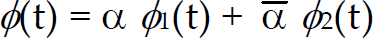
As it is shown in Fig. 7, a Boolean variable α has been introduced to be used as a switch between the two FLC employed to achieve the oriented positioning. Initially, α is equal to “1”, so that the RPC works first. Once the Sub-goal reached, α turns to “0” in order to select the RFC. By this way, the two controllers used for oriented positioning are working in serial. The controller's output variables are obtained from the following equations:

$$v(t)=\alpha v1(t)+\bar{\alpha }v2(t)$$

(9)

$$\varphi (t)=\alpha \varphi 1(t)+\bar{\alpha }\varphi 2(t)$$

(10)

The used FLCs have been tested in simulation, with Simulink of Matlab 6.5, then implemented in real-time with C++ under Linux Redhat 6. In the next section, simulation results of simple positioning are exposed and commented.

2.3 Simulation tests

To test and demonstrate the effectiveness of the proposed strategy, a computer simulation has been performed. For that, simple positioning is implemented on a car-like kinematic model. In all tests, robot's localization is computed by Incremental Odometer. Initial configuration of the robot is taken in the origin O(0m, 0m, 0°). This choice is not a necessary condition to get a convergence. We start testing simple positioning FLC.

In Fig. 9, four goals are chosen with the following coordinates (in meter) : T₁(8,9), T₂(−16,14), T₃(−7,−13), and T₄(12,−12). The test shown in Fig. 9(a) has been done as follow: the robot starts moving from the initial position O(0,0) then goes to T₁. Once arrived, it starts to move toward T₃. After that, it is directed toward T₂ and finally T₄ where it stops. This test has been made to verify that the RPC controller functions correctly from any initial position to any desired goal, with both positive and negative coordinates. In the second test shown on Fig.9(b), the robot moves on a closed trajectory which starts and ends on the origin as follow:

$$(\mathrm{O}\to {\mathrm{T}}_3\to {\mathrm{T}}_2\to {\mathrm{T}}_1\to {\mathrm{T}}_4\to {\mathrm{T}}_3\to \mathrm{O})$$

Fig. 8.

Flowchart of oriented positioning.

Fig. 9.

Simple positioning robot trajectories.

The robot converges without any problem. From the first test, the control variables v and φ are measured when the robot was moving from the origin O(0m,0m,0°) to T₁. Fig.10(a) illustrates the variations of the robot's velocity v during the simple positioning. We can see that the velocity variation is continuous and kept under limits (less than 3m/s). When the robot arrives to the goal, velocity is near to “zero”.

Fig. 10.

Control variables in simple positioning.

In Fig. 10(b), the variation of the steering angle φ when the robot is moving to T₁ is shown. Even if the initial value is important (≈ 14°), it does not disturb the robot because velocity v is small at this moment. In addition, the big variation of the steering angle φ (from 0° to 16°) between t=10s and t=15s does not disturb the movement of the robot, because velocity is small too. In all tests, robot stability and security was guaranteed by the used controllers.

Simulation results of oriented positioning are presented and compared to the experimental results in section 3.

3. Experiments

The proposed strategy for oriented positioning has been implemented on a car-like mobile robot called Robucar (Fig. 11).

Fig. 11.

A photograph of the mobile robot Robucar

The Robucar is a nonholonomic mobile robot designed by INRIA (France) and manufactured by Robosoft (Laugier & Parent, 1999). It is equipped by optical encoders for localization, LMS and US sensors for obstacle detection and CCD camera for visual perception. Tests have been done in indoor and outdoor environments for many goals, chosen with usual orientation (0°, 45°, 90°, 180°) to make easy results verification. Fig. 12 shows trajectories for the goal T₅ (11,6)m with different orientations as follow:

$$(\mathrm{a}\to -{90}^{\circ },\mathrm{b}\to 0^{\circ },\mathrm{c}\to {90}^{\circ },\mathrm{d}\to {180}^{\circ }).$$

Fig. 12.

Oriented positioning trajectories for goal T₅

The Fig. 13 shows robot trajectories for the goal T₆ (−10,8)m with the following orientations:

$$(\mathrm{a}\to {45}^{\circ },\mathrm{b}\to -{45}^{\circ },\mathrm{c}\to {135}^{\circ },\mathrm{d}\to -{135}^{\circ })$$

Fig. 13.

Oriented positioning trajectories for goal T₆

A comparison between control variables variations in simulation and in real-time implementation, of the oriented positioning task, from the origin O(0m,0m,0)) to goal T₇(10m,12m,−30°) is shown on Fig. 14. Velocity variations are similar in both: differences are negligible and might be due robot-ground interactions in real tests (Fig. 14(a)). The same remarks can be done on Fig. 14(b), where the variation of the steering angle is the same in simulation and in experimental test. From all these results, we can say that the effectiveness of the proposed strategy is verified for any oriented goal T(X_G Y_G θ_G).

Fig. 14.

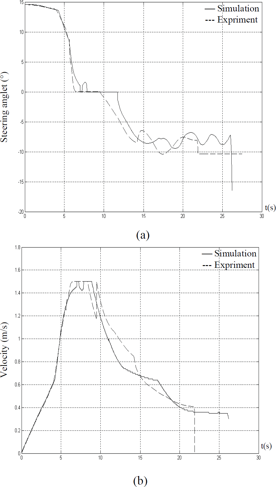
Control variables in oriented positioning

4. Conclusion

This paper presents a new technique used to perform the task of Oriented Positioning on a nonholonomic mobile robot, using two fuzzy logic controllers. The first controller used for Simple Positioning has been implemented and tested on simulation. Then, it is combined with a second controller, used for “Virtual Following”, in order to accomplish the desired task. Realtime experimentations have been performed on the carlike mobile robot “Robucar”. Obtained results show the effectiveness of the proposed techniques. It is guessed that if this technique is enhanced by introducing obstacle avoidance, it can be of interest for developing new autonomous transportation ways. So we are focusing our works on implementing an obstacle avoidance task by using fuzzy logic or neural networks.