
Abstract
In this paper differential kinematics was geometrically derived to be utilized in a calibration algorithm that improves the accuracy of the manipulation of a robot. Even though the mechanical components are manufactured and assembled precisely, small differences between the designed and the actual system always exist, due to both geometric and unmodelled errors. In order to resolve these problems, differential relationships between the model parameters and the end-effector's posture were formulated. Subsequently, a derivative based estimation algorithm, such as an EKF (Extended Kalman Filter) manner, could be adopted to update the model parameters. The proposed algorithm includes joint flexibility, so is an advanced version of previous work, where a rigid joint model was adopted [1]. The effectiveness of the proposed algorithm was verified by a computer simulation with a 6 DOF manipulator robot.
1. Introduction
Obtaining information concerning the links and the joints of a manipulator is essential for the control of robotic systems. Especially in research involving an articulated link manipulator, which consists of a series of links, such as a robotic arm, finger, or leg and where the accuracy of the model directly influences the performance of the task. Since the model parameters determine the mathematical model, it is important to gain parameters that are as accurate as possible. Although 3D CAD tools provide accurate information about a model, the geometry of the manufactured robot is not generally identical to the designed one. Consequently, the differences reduce the performance of the manipulation significantly. These inaccuracies in the model parameters of the robotic systems arise from two kinds of errors: geometrical and unmodelled errors. The geometrical errors are caused by inaccurate manufacturing, assembling, etc. The unmodelled errors are commonly caused by the approximation of the mathematical formulation, such as the joint flexibilities, thermal dynamics, etc. Therefore, in order to improve the performance and/or the stability of the manipulation, it is necessary to calibrate the model parameters as well as utilizing the advanced model.
There has been a lot of research related to the kinematical identification and calibration of manipulator robots. A methodology that uses lasers was introduced to capture robot position data in order to model the stiffness of the robot manipulator [2] and to predict kinematic parameters [3, 4, 5, 6, 7]. O'Brian et al. also employed magnetic motion capture data to determine the kinematic parameters [8]. Renaud et al. [9] and Rauf et al. [10] used a vision-based measuring device and a partial pose measurement device, respectively, for the kinematic calibration of parallel mechanisms. Gatti and Danieli demonstrated a pose-matching procedure for calibration, which provided a low cost and easy-to-use external metrology system [11]. Santolaria et al. recently demonstrated a continuous data capture technique by using a ball bar gauge and a coupling probe to estimate the kinematic parameters of articulated arm coordinated measuring machines [12]. It was concluded that the parameter error was minimized in the measured positions, whereas the error increased in very different positions because the optimization technique was only based on the position information of the end-effector. To overcome this problem, Ye et al. [13] and Iurascu and Park [14] demonstrated a kinematic calibration method using differential kinematics and iterative algorithms to determine the parameters.
In the previous research, a novel algorithm was proposed to estimate the entire kinematic parameters of the robot manipulator by using a structured laser module (SLM), a stationary camera and a screen [1]. In the algorithm, by using the Jacobian matrix, which represents the relationship between the kinematical parameters and the laser points on the screen, an iterative estimation scheme, such as the extended Kalman filter (EKF), was adopted. For the kinematic model, Denavit-Hartenberg (D-H) convection is used and all the joints and the links were modelled as rigid. In this paper, the previous method was extended by employing the flexible joint model. To improve the accuracy of the manipulation, three types of model parameters were estimated: the D-H parameters, the joint compliances and the CM positions of the links. Similarly to previous work, an SLM system with a stationary camera and a screen was adopted to estimate the model parameters. The performance of the proposed algorithm was verified with a 6 DOF humanoid leg system by computer simulation.
This paper is organized as follows. In Section 2, problems concerning a flexible joint model are defined and described. Subsequently, in Section 3 and 4, mathematical models and Jacobians are discussed. In Section 5, the effectiveness of the proposed algorithm is verified by simulation results. Lastly, concluding remarks follow in Section 6
2. Problem Definition
In order to control a robot manipulator precisely, it is essential to know the model parameters of the manipulator. However, there are always some errors in link lengths and link twists during manufacturing and/or assembling the robot system. These undesirable errors reduce accuracy during the manipulation and sometimes make the system unstable. They may cause more problems in a complex articulated linkage system such as a humanoid robot. Small errors in each joint accumulate and eventually make a significant difference between the model and the actual system.
In previous work, a novel systematic algorithm was introduced to measure the errors in the kinematical parameters by using a structured laser module (SLM) and a stationary camera system. Using the algorithm, the kinematical errors were successfully measured; thereby it enhanced the accuracy of the forward and inverse kinematics. Since the algorithm uses a lot of standstill manipulator postures in the rigid kinematical model, when the mass of the link of the manipulator is large or the stiffness of the joint is small, differences between the computed and the measured points increase significantly because of the influence of gravitational force. These are represented in Fig. 1, where θ and φ represent the controlled joint angle in the rigid model and the additional rotation in the flexible model, respectively and τg represents gravitational torque. Note that in the rigid model φ is assumed to be zero, while it has a significant value in the flexible model.

Influence of the joint flexibility.
In order to estimate the model parameters, a similar measurement system is introduced as shown in Fig. 2. The proposed system consists of a SLM attached to a manipulator, a stationary camera and a screen. Note that the base frame is attached to the screen and the stationary camera is used to measure the position of the laser point on the screen. When all the kinematical parameters, including joint compliances and mass positions, are accurately known the computed laser points on the screen for the given robot posture must be identical to the actual points measured by the stationary camera. Since there are some model errors, this generally does not happen as mentioned above. The proposed method uses the differences between the computed laser points with the current estimated parameters and the actual measured points to update the parameters. While doing this, the differential relationships, known as the Jacobian matrix, are utilized. A detailed mathematical model and derivation of the Jacobians are described in Section 3 and 4. Note that this paper focuses on how to derive Jacobians geometrically. Its applications, including experimental analysis, will be treated in further work.

System configuration to calibrate the model parameters.
3. Mathematical Model
D-H convention is adopted to describe the kinematics because it requires a minimum number of parameters to represent the coordinate system attached to each link, as shown in Fig. 3. Here α and β are the joint offset angle and the twist angle between the joint axes and d and l are joint distance and link length, respectively. Lastly, θ and φ are the controlled joint angle and the deformed twisting angle due to the flexibility.

D-H convention for coordinate frame system.
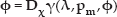
From the D-H parameters and the twisting angles caused by the joint flexibility, the end-effector's posture is determined as follows:

where λ and φ are 4(n+1) × 1 vector for the D-H parameters and n × 1 vector for the twisting angles, respectively and ∂e is a 6 × 1 vector that consists of a position (

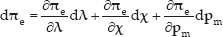
In a stationary state, the twisting angles can be represented by the following implicit function:

where χ and

where γ and
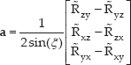
By solving Eq. (5) algebraically for dφ (differential relationship among the compliances), the D-H parameters and the mass positions are obtained as follows:

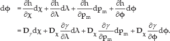
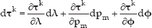
By substituting Eq. (6) into Eq. (2), differential kinematic motion is finally expressed with differentials of the D-H parameters. The compliances and the mass positions are as follows:
where

Eq. (7) represents the relationship of the infinitesimal displacements among the kinematical parameters, the compliances and the mass positions for the end-effect posture. By applying a derivative based estimation algorithm such as Least-squares manner or Extended Kalman Filter, the model parameters can be effectively calibrated. The overall algorithm is summarized in the block diagram in Fig. 4. In forward kinematics, the coordinate frames

Block diagram of overall algorithm flow.
Algorithm 1 describes how to compute twisting angles iteratively. After initialization, Homogeneous Transformation Matrices are computed with the given joint coordinates, the model parameters and the kth twisting angles. Subsequently, from the kinematical configuration, joint torques can be obtained by static equilibrium condition. Since the joint model in this paper assumes that the compliance coefficient is constant, the twisting angles are easily calculated and updated. If the norm of the difference between the kth and the (k + 1)th twisting angles is small enough, the (k + 1)th twisting angles are saved and the iteration is terminated. After the forward kinematics stage, the Jacobian matrices are computed. Note that the derivations of the Jacobians in Eq. (7) will be described in detail in Section 4. Subsequently, the Least-squares method or EKF is utilized to update the model parameters, the D-H parameters λ, the compliances χ and the CM positions
Compute twisting angles under joint flexibility

4. Geometrical Derivation of Jacobians
4.1 Jacobian for the End-Effector Posture from the D-H Parameters and the Twisting Angles.
From Eq. (7), the Jacobian matrix for the end-effector posture from the model parameters consists of partial derivatives as follows:

Since the Jacobian matrix accompanies partial derivatives, it is generally hard to compute analytically. Fortunately, however, for the articulated linkage system, it can be computed geometrically. The Jacobian matrix is computed using exactly the same manner as the general kinematics, except that the parameters are the D-H parameters λ = [··· α k dk lk βk ···]T and the twisting angles φ = […φk…]T, not the joint angles θ = [···θk···]T, as shown in Fig 5.

Coordinate frames for Jacobian Computing
The Jacobian is comprised by differential translations and rotations with respect to the corresponding parameters. The differential translations and rotations by translational parameters such as dk and lk are simply unit vectors in the direction of the translations and zero vectors. Also, the differential translations and rotations by the rotational parameters, such as αk, βk and φk, are a cross product of rotational axis vectors and distance vectors, respectively. Eq. (9) represents these formulas.


4.1.1 Partial Derivatives for the D-H parameters
By applying Eq. (9), the partial derivatives of the end-effector posture for the D-H parameters are computed as Eq. (10).
4.1.2 Partial Derivatives for the twisting angles
In a similar manner, the partial derivatives of the end-effector posture for the twisting angles are computed as follows:

4.2 Derivatives of the Joint Torques for the D-H Parameters, the Twisting Angles and the CM Positions
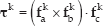
The laser pointers on the screen are measured during standstill state. Consequently, the torques applied to each joint are determined from the gravitational force only. Fig. 6 illustrates the coordinate frames and the CM positions for the revolute joints. Note that the kth joint torque, τk, is affected from the kth link to the last link.

Coordinate frames and CM positions for revolute joints
The effective CM position, which is the average value from the kth link to the last link, is calculated as follows:
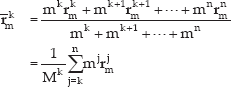
where
with


where
By differentiating Eq. (13), the differential of the joint torque for the D-H parameters, the CM positions and the twisting angles are derived as follows:
Where detailed partial derivatives are given as follows:


From Eq. (11), (12), and (16), the Jacobian matrix, Eq. (8), can be computed sequentially.
4.3 Comparison with numerical computation method
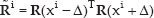
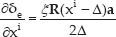
So far, the Jacobian matrix between the model parameters and the end-effector posture is geometrically derived. An alternative approach for the Jacobian derivation is to use numerical differentiation. Using the definition of the Jacobian matrix, it can be divided into two parts: position derivative and orientation derivative, as follows:

where

where xi is the ith value of
where
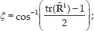
where tr(·) represents a trace operation. The axis vector is derived as follows:
From Eq. (20) and (21), the orientation derivative is numerically derived as follows:
In Table 1, the accuracy of the numerically derived Jacobian is compared with the geometrically derived Jacobian. For quantitative analysis, 1000 test postures were selected and Jacobian matrices were computed according to the above two methodologies. Subsequently, the results were analysed in a statistical manner. From the table, it can be shown that both approaches give similar results. This implicitly guarantees that the geometrical formula is correctly derived and thus it gives true values. Practically, numerical derivation sometimes suffers from the division by zero problem.
Errors of the numerical Jacobians

Another important benefit of using geometrical derivation is computing time. Since the numerical derivation utilizes two different postures deviated by Δ to obtain one column of Jacobian matrix, ∂∂e / ∂xi, it requires a much greater computational process. From the simulation results, it can be seen that it takes 10.0622 seconds for 1000 calculations of geometrical derivation and 249.005 seconds for 1000 calculations of numerical derivation using Matlab. Using the geometrical derivation of a Jacobian matrix reduces the run time for the calibration algorithm dramatically.
4.4 Jacobian for the laser points on the screen from the end-effector
After obtaining the relationships from the kinematical parameters, including the compliances and the CM positions of the end-effector posture, the relationship between the end-effector posture and the laser points projected onto the screen must be found. From [1], the Jacobian matrix of the laser point on the screen from the end-effector is given by:

where

From Eq. (8) and (23), the final Jacobian matrix is derived as follows:

Note that the Jacobian matrix is the relationship of the differential motions between the model parameters and the laser points on the screen.
5. Computer Simulation
The effectiveness of the derived Jacobians was verified by adopting a computer simulation with a 6 DOF humanoid-legged robot, as shown in Fig. 7. To calibrate the model parameters, 100 test postures were selected by arbitrarily choosing joint angles between −20 and +20 degrees. Subsequently, the laser pointers on the screen corresponding to each posture were obtained. An initial guess for the D-H parameters is randomly selected between 80% and 120% of the true value and random noise between −0.02 to +0.02 is added. The rest of the model parameters for the initial guess are randomly selected between 90% and 110% of the true value and random noise is added between −0.01 and +0.01. Also, during the measurement of the laser points on the screen, random noise between −0.001 to +0.001 was added. Note that the coordinate frame for the 1st laser in SLM, σl1, coincides with the coordinate frame for the 6th link, σ6, while the coordinate frames for the 2nd and the 3rd lasers, σ12 and σ13, are rotated by +30 and −30 degrees about the x-axis, respectively and are followed by a rotation of +10 degrees about the y-axis. Detailed model parameters used in the simulation are summarized in Table 2.
Model parameters (true values).


Coordinate frames of a 6 DOF leg robot.
In order to verify the effectiveness of the flexible joint model, the rigid joint model (previous work) was also examined. For EKF, both the covariance matrix of system noise and measurement noise were set as 1.0×10⁴ for D-H parameters and 1.0×10⁶ for the rest of the model parameters. The simulation was carried out using the Matlab program on Intel core i5–2500 CPU at 3.30 GHz with 4.0 GB RAM. The simulation takes 10.6 seconds for the rigid model and 146.5 seconds for the flexible model, respectively. Note that the total number of model parameters to be calibrated is 28 (excluding compliances and CM positions) for the rigid model and 52 for the flexible model.
5.1 Simulation with rigid joint model
In the rigid joint model, the Jacobian matrix of the end-effector's posture is a function of D-H parameters only. Consequently, the differential kinematic motion in Eq. (7) is simplified.

From Eq. (25), EKF was iteratively executed with the same manner as in the previous work [1], except that compliance was taken into account in the measurement of the laser points on the screen. Convergence of the EFK and the model parameters is shown in Fig. 8 and Fig. 9, respectively.

Convergence of EKF (rigid model).

Divergence of model parameters (rigid model).
Although the EKF converged, the estimated model parameters could not converge as expected because the algorithm could not handle the joint flexibility. In other words, the EKF reduces the number of measurement errors by manipulating the D-H parameters to compensate the compliance effect. Consequently, the D-H parameters grow away from the true values.
5.2 Simulation with flexible joint model
The proposed algorithm was simulated with the same conditions. As shown in Fig. 10 and Fig. 11, the EKF and the model parameters converged.

Convergence of EKF (flexible model).

Convergence of model parameters (flexible model).
In order to investigate whether or not the estimated model parameters are effective on arbitrary postures as well as the test postures, 20 new test postures were created and examined, as shown in Fig. 9. Test postures were generated as follows:

where θ k (k = 1,···,20) represents the joint angles for the test postures and qk is the kth angle from 0 and 2∂.
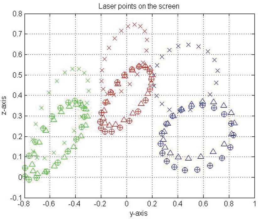
Laser points on the screen with test postures.
The ‘○’ markers and the ‘×’ markers represent the laser points on the screen with the true model parameters and the initial guess, respectively. The‘+’ markers indicates the laser points after calibration using the flexible joint model (proposed algorithm), while the ‘Δ’ markers correspond with the rigid joint model (previous algorithm). As shown in the figure, every calibrated point using the flexible joint model nearly coincides with the true points, whereas the calibrated points from the rigid joint model are located further apart from the true points.
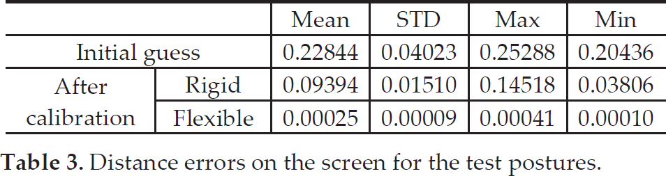
In Table 3, the distance errors between the true points and the two calibrated points were compared with the errors between the true points and the non-calibrated points with the initially guessed parameters. As shown in the table, the accuracy was improved in every category.
Distance errors on the screen for the test postures.
6. Conclusion
In this paper, differential kinematics of a flexible manipulator were geometrically derived to calibrate model parameters such as the D-H parameters, the joint compliances and the mass positions. From a practical point of view, the proposed geometrical manner was compared with a numerical derivation technique. The proposed manner is not only free from the division by zero problem, but also much faster. In addition, by adopting the differential kinematics into a calibration system composed of a laser and a camera, the model parameters were iteratively updated. Consequently, the difference between the measured and the computed laser points on the screen was effectively decreased. A computer simulation with a 6 DOF humanoid-legged robot was carried out and confirmed that the proposed algorithm could calibrate the model parameters automatically. Applying the algorithm to actual robotic systems is an area for further work.