Sage Journals: Discover world-class research

Abstract

Unstructured road detection is a key step in an unmanned guided vehicle (UGV) system for road following. However, current vision-based unstructured road detection algorithms are usually affected by continuously changing backgrounds, different road types (shape, colour), variable lighting conditions and weather conditions. Therefore, a confidence map of road distribution, one of contextual information cues, is theoretically analysed and experimentally generated to help detect unstructured roads. Two traditional algorithms, support vector machine (SVM) and k-nearest neighbour (KNN), are carried out to verify the helpfulness of the proposed confidence map. Following this, a novel algorithm, which combines SVM, KNN and the confidence map under a Bayesian framework, is proposed to improve the overall performance of the unstructured road detections. The proposed algorithm has been evaluated using different types of unstructured roads and the experimental results show its effectiveness.

Keywords

Unstructured Road Detection Confidence Map Of Road Distribution Support Vector Machine K-Nearest Neighbour Algorithm

1. Introduction

Road detection is a key requirement for unmanned guided vehicles (UGV). Paved road following is largely considered a “solved” problem, as a lot of approaches for road following have been proposed and successfully demonstrated in the last two decades [1 –3]. Although this topic has already been documented in technical literature by different research groups, unstructured road detection poses several interesting and new challenges due to its unstructured nature [4, 5]. For example, the road edge border may be unclear and it may have a low intensity contrast. Additionally, the overall road shape may be arbitrary, which leads to a road surface with a degraded appearance. Furthermore, varying illumination conditions, different viewpoints and changing weather conditions make the problem more complex [6]. As shown in Fig.1, different illumination and different weather conditions change the same scene into various different texture properties. In all of these conditions, many road following systems would fail because the road feature extraction is difficult and the detection becomes inaccurate.

Figure 1.

The same scene in different lighting conditions, different weather conditions and from different viewpoints.

Many algorithms have been proposed to deal with unstructured road detection in recent decades. The previous methods can be mainly divided into three groups: the model-based method [7, 8], the feature-based method [9], and the machine learning-based method [10, 11]. However, current vision-based methods are usually based on low-level features [12]. For example, HSV colour feature is used in [7, 13], while an improved RGB colour feature is chosen in [14]. Recently, feature-combination methods have been widely researched. Three features of a lane boundary starting position, direction and grey-level intensity features comprise a lane vector via simple image processing in [15]. Additionally, in order to improve the effectiveness of road detection under different conditions, contextual information is first used in addition to low-level cues in road detection [16]. Though the results in [16] show its algorithm is effective, the paper did not give any details of contextual information in theory, how to generate it or how much this contextual information had improve the road detection results.

Therefore, in this paper, we specifically discuss the process of generating a confidence map of the road distribution - theoretically and experimentally. Following this, in order to show the helpfulness of the proposed confidence map, experiments are carried out by using traditional support vector machine (SVM) and k-nearest neighbour (KNN) algorithms. In both of these two algorithms, a typical low-level feature named the histogram of RGB value is used. Finally, a novel algorithm, which is different compared with traditional feature-combined methods, by combining SVM, KNN and a confidence map under a Bayesian framework is proposed to improve the overall performance of the unstructured road detection. Experiments show the proposed algorithm is effective.

The remainder of this paper is organized as follows. In Section 2, we theoretically analyse the distribution probability of the road and then deduce a confidence map experimentally. In Section 3, two algorithms, the SVM-based and the KNN-based road detection algorithms are applied to show whether the proposed confidence map is helpful during the road detection. In order to implement the SVM and the KNN algorithms, a typical low-level feature named the histogram of RGB value is introduced in this paper. Furthermore, a novel algorithm which combines SVM, KNN and a confidence map under a Bayesian framework is proposed in this section. Section 4 illustrates the details of experiments under various road conditions and compares these to state-of-the-art methods. The results show that the proposed confidence map greatly enhances the ability of unstructured road detection, and that the proposed novel algorithm is effective. Section 5 concludes the paper.

2. Analysing the distribution of the road

Contextual information is considered very helpful to road detection [16], however, paper [16] did not give any theoretical details of contextual information, how to generate it or how much this contextual information improved the road detection results. In this section, the distribution information of the road is theoretically analysed and experimentally generated. Some factors which affect the distribution of the road are discussed. Following this, a series of confidence maps are generated using an evaluation platform. Finally, a policy to choose the corresponding confidence map is simply introduced by using global positioning system (GPS) information.

2.1. Mapping from world coordinates to the image frame buffer

To get an explicit description of the appearance of the road surface in the frame buffer and to illustrate the projection from 3D space (vehicle coordinates) to the 2D space (frame buffer coordinates) in a simple way, we first define some required coordinates (Fig.2): the frame buffer (c,r)in pixels, the image coordinates (X_I,Y_I) in metres, the camera coordinates (X_C,Y_C,Z_C) in metres, and the vehicle coordinates (X_V,Y_V,Z_V) in metres.

Figure 2.

Coordinates in our system: (X_V, Y_V, Z_V) are the vehicle coordinates; (X_C,Y_C,Z_C) are the camera coordinates; cr are the pixel coordinates and (X_I, Y_I) are the image coordinates; θ is the pitch angle of the camera.

The appearance (coordinate values) of the lane in the digital image of the road scene can be obtained as a transformation from the 3D Euclidean space of the vehicle coordinates to the 2D Euclidean space of the frame buffer. In practice, the transformation can be divided into two stages: the first stage is the transformation from the world coordinate system to the camera coordinate system, and the second stage is the projection from the camera coordinate system to the image frame buffer.

The transform from the vehicle coordinates to the camera coordinates can be expressed as:

^{C} P =_{V}^{C} R (^{V} P +^{V} P_{C})

(1)

The rotation transformation ${}_{V}^{C}R$ can be achieved by the Euler angles. The shift transformation ^VP_C is the offset of the optical centre in the vehicle coordinates. All the parameters considered here are determined by the extrinsic parameters of the on-board camera. Usually the onboard camera of the road detection system is mounted on the vehicle with careful design. It is reasonable to assume the offset of the optical centre in the vehicle coordinates to be (0,0,h) and the rotation angles from the vehicle coordinates to the camera coordinates to be (0, π /2 + θ, 0). Equation (1) can be expressed as

[\begin{matrix} X_{C} \\ Y_{C} \\ Z_{C} \end{matrix}] = [\begin{matrix} 1 & 0 & 0 \\ 0 & c o s (π / 2 + θ) & s i n (π / 2 + θ) \\ 0 & - s i n (π / 2 + θ) & c o s (π / 2 + θ) \end{matrix}] [\begin{matrix} x_{V} \\ y_{V} \\ z_{V} - h \end{matrix}]

(2)

If we omit the distortions of the lens, the projection can be expressed as:

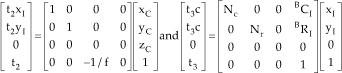
[\begin{matrix} t_{2} x_{I} \\ t_{2} y_{I} \\ 0 \\ t_{2} \end{matrix}] = [\begin{matrix} 1 & 0 & 0 & 0 \\ 0 & 1 & 0 & 0 \\ 0 & 0 & 0 & 0 \\ 0 & 0 & - 1 / f & 0 \end{matrix}] [\begin{matrix} x_{C} \\ y_{C} \\ z_{C} \\ 1 \end{matrix}] and [\begin{matrix} t_{3} c \\ t_{3} c \\ 0 \\ t_{3} \end{matrix}] = [\begin{matrix} N_{c} & 0 & 0 & ^{B} C_{I} \\ 0 & N_{r} & 0 & ^{R} B_{I} \\ 0 & 0 & 0 & 0 \\ 0 & 0 & 0 & 1 \end{matrix}] [\begin{matrix} x_{I} \\ y_{I} \\ 0 \\ 1 \end{matrix}]

(3)

Furthermore, if we combine all the steps of the transformation into one expression, the perspective projection from the 3D vehicle coordinate to the 2D frame buffer can be expressed as:

{\begin{array}{l} c =^{B} C_{I} + \frac{x_{v}}{c_{f} ((z_{v} - h) s i n (θ) + y_{v} c o s (θ))} \\ r =^{B} R_{I} + \frac{(z_{v} - h) c o s (θ) + y_{v} s i n (θ)}{r_{f} ((z_{v} - h) s i n (θ) + y_{v} c o s (θ))} \end{array}

(4)

Where, $c_{f} = \frac{1}{N_{c} f}$ and $r_{f} = \frac{1}{N_{r} f}$ represent the actual length of one pixel divided by the focus length. N_c and N_r are the distances between two adjacent pixels on the sensor in the horizontal and vertical directions. ^BC_I and ^BR_I are the coordinate values of the optical center in the frame buffer.

2.2. Parameter representation of the lane in the vehicle coordinates

A curved road model in the vehicle coordinates can be expressed as:

{\begin{cases} x_{v} (t) = c_{0} + t a n (ϕ) t + c_{2} t^{2} \\ y_{v} (t) = t \\ z_{v} (t) = 0 \end{cases}

(5)

Here, t is the arc length along the running direction of the vehicle. c₀ is the lateral offset of the vehicle relative to the road. c₁ = tan(φ) is the tangent of the heading angle of the vehicle relative to the local direction of the road. C₂ is the curvature parameters of the road.

Putting equation(5) into (7), the refined perspective projection transformation from the 3D vehicle coordinate to the 2D image frame buffer is:

{\begin{array}{l} c =^{B} C_{I} + \frac{c_{0} + t a n (ϕ) t + c_{2} t^{2}}{c_{f} (s i n (θ) h + c o s (θ) t)} \\ r =^{B} R_{I} + \frac{c o s (θ) h + s i n (θ) t}{r_{f} (s i n (θ) h + c o s (θ) t)} \end{array}

(6)

Where the φ is considered very slight. We list the factors that affect the position of the road surface in the road image as follows:

Heading angle of the vehicle φ;

Pitch angle of onboard camera θ;

The curvature parameters of the road c₂.

The actual length of one pixel divided by the focal length of the onboard camera cf and r_f.

When a camera is fixed, the last two factors, c_f and r_f, can be assumed constant. The parameter c₂ is decided by actual road path. The variation of pitch angle θ is caused by changes in the pitch angle of the vehicle. The heading angle φ is caused by the variation in vehicle manoeuvres.

2.3. Creating the confidence map from the evaluation platform

We have theoretically analysed the factors that influence the position of the road surface above. For simplification, we model the three factors as i.i.d. random variables with 1D Gaussian distribution

ϕ \sim N (ϕ_{0}, σ_{ϕ}), θ \sim N (θ_{0}, σ_{θ}) and c_{2} \sim N (c_{2_{0}}, σ_{c_{2}}) .

When the onboard camera is fixed, both the extrinsic and intrinsic parameters of the camera are fixed. Assum φ ϵ [-10°, 10°, 10°], θ ϵ [-5°, 5°] and the road curvature radii from 250m to infinite. According to (6), using variance (ϵ_φ, ϵ_θ,ϵ_c2) to set the search range for the actual road surface, a series of images can be generated by an evaluation platform (Fig. 3). The evaluation platform is offered by [17].

Figure 3.

Series of road images generated by the evaluation platform.

These parameters are thought to be independent and as i.i.d. random variables with 1D Gaussian distribution. These images are added together according to different road curvatures under the guide of 1D Gaussian distribution. Thus, a series of confidence maps with corresponding different curvatures are generated (Fig. 4).

Figure 4.

A series of confidence maps corresponding to different road curvatures. A deeper colour refers to the higher probability of road surface.

2.4. Selection of a suitable confidence map

GPS information is widely used to locate a vehicle in the global map during its derivation [1]. A real-time dynamic differential GPS could locate a vehicle accurately with a precision at the one centimetre level if enough information from several satellites is available. Unfortunately, in most areas with dense urban environments (e.g., buildings and thick trees), the GPS error is at the metre level or even worse. In this work, we use the GPS information to locate the vehicle simply. In this case, the road direction in front of the vehicle can be obtained, after which the corresponding confidence map is chosen to improve the road surface detection. As shown in Fig.5, the triangle means the position of the vehicle located by GPS, and the circle means the error region. In this case, the road curvature in front of the vehicle is known and the corresponding confidence map is chosen.

Figure 5.

GPS information helps to select the confidence map.

3. Verifying the usefulness of the confidence map

In order to verify whether the confidence map is useful during the road detection, two traditional algorithms, SVM and KNN, are applied in this section. A typical local feature named the histogram of RGB value is introduced and used in these two feature-based algorithms. Finally, a novel algorithm which combines SVM, KNN and the proposed confidence map together under a Bayesian framework is proposed to improve the effectiveness of road detection.

3.1. The histogram of RGB values

A lower feature descriptor is necessary both in SVM-based and KNN-based road detection algorithms. The RGB colour space has been extensively tested and used in previous road tracking applications on unstructured roads [7, 14]. A typical feature descriptor named the histogram of RGB value, which is similar to the histogram of orientation gradient (HOG) [18], is introduced and used both in SVM and KNN to show the helpfulness of the proposed confidence map in our experiments.

The definition of the histogram of RGB values is similar to histogram of orientation gradient (HOG) [18], given that they capture local shape information by encoding RGB gradients in histograms. In each colour channel, pixels are divided into n bins. The count of each bin is used as the input feature. The advantage of this feature descriptor is that different textures in an image will express themselves differently in histograms [8].

In our experiment, the count of every bin in each colour channel is 8, thus the vector size of the RGB histogram is 8 × 3 = 24.

A set of positive samples and a set of negative samples are generated from the variable road surface and background chosen by human selection. These two sets are shown in Fig.6. The count of training images is about 1/1000 of total test images in each type of roads. The details of experiments will be described in Section 4.

Figure 6.

The sets of training samples.

The process of using the histogram of RGB values in the SVM algorithm or in the KNN algorithm can be summarized as follows: the original image is first divided into several windows. The size of each window in our experiments is 10 × 10. In each window, the histogram of 100 pixels in each channel is computed. The number of bins in our experiments is 8. Therefore, the histogram of RGB value is a 1 D vector, whose size is 8 × 3 = 24. This 1D vector is used as a feature parameter, both in the training step and in the recognizing step.

3.2. Support vector machine

SVM is a technique motivated by statistical learning theory, which has shown its ability to generalize well in high-dimensional space [14]. The key idea of SVM is to separate two classes with an optimal decision hyper-plane of the maximum margin. Traditionally, the classifier returns property “+1” (this refers to a road region) or “-1” (which describes the background). We use the margin distance instead of that property, in which pixels with longer distances (a deeper colour in the pictures) will exhibit higher probability of being road pixels.

The SVM structure is trained off-line by using training samples. The result of the road detection by SVM is shown in Fig.7. The upper row is the benchmark marked by humans, the second row is the margin distance detected by SVM, the third row is the result when an optimum threshold (threshold = 0.5) is chosen, and the lower row is the result achieved with the help of the proposed confidence map. We define the true positive rate as TP=P_d/P_bk, and the false positive rate as FP - F_d/P_bk. P_d is the pixel number in the road region detected by a method. P_bk is the pixel number of road region in the benchmark. F_d is the pixel number out of the road region but detected by the method as road surface. When an optimum threshold = 0.5 is chosen, the true positive rate of the SVM-based algorithm is TP_svm −85.49%, and the false positive rate is FP_svm = 8.61%.

Figure 7.

road detection by SVM. The upper row is the benchmark marked by a human, the second row is the margin distance detected by SVM, the third row is the result of road detection when an optimum threshold (threshold = 0.5) is chosen, the lower row is the result under the help of the proposed confidence map. In the last two cases, green pixels refer to road regions.

On the other hand, the proposed confidence map is used during the road detection process according to the equation: P(x_i = R|P_svm) = P_svm P(x_i = R). P(x_i = R) is the confidence map for a pixel x_i depicting the road surface, whilst P_svm means the result of road detection by SVM. With the help of the corresponding confidence map, TP_svm+map =96.82%, and FP_svm+map = 10.63%. It is clear tha_svm+map proposed confidenc map greatly improves the true positive rate of the road detection, though the false positive rate is also slightly improved.

3.3. K-nearest neighbour

The KNN algorithm is a classical texture classification algorithm. K cluster centres are trained by the positive data set. During the detection, each pixel in the original image will have a minimal distance to these k cluster centres. The distance means a similar rate between new pixels and road regions.

In our experiments, 20 cluster centres are used, which are trained off-line by using the positive samples. The result of the road detection by KNN is shown in Fig.8. The upper row is the distance value detected by KNN, the middle row is the result when an optimum threshold (threshold = 18) is chosen, and the lower row is the result with the help of the proposed confidence map. Under the same conditions, when the optimum threshold is chosen, the true positive rate of KNN is TP_knn = 91.83% and, the false positive rate is FP_knn = 11.06%. In the same way, with the help of the corresponding confidence map, the result of road detection is TP_knn+map = 97.45% and FP_knn+map = 10.42%. It is clear that the proposed confidence map greatly improves both the true positive rate and the false positive rate of the road detection.

Figure 8.

Road detection by KNN. The upper row is distance value detected by KNN, the middle row is the result of road detection when an optimum threshold (threshold = 18) is chosen, the lower row is the result under the help of the proposed confidence map. Again, in the last two cases, green pixels refer to road regions.

3.4. ROC shows the effectiveness of the confidence map

The ROC (receiver operating characteristic) curve is used to show the improvement of the proposed confidence map compared with the traditional single SVM or single KNN algorithm. ROC curve reflects the true positive rate against the false positive rate while shifting the threshold in a fixed range. A series of different types of unstructured road scenes under various lighting conditions and different weather conditions were tested (the details of the experiments are described in Section 4). The threshold range of SVM is [0.2, 1] and the threshold range of KNN is [2, 50]. In Fig.9, the blue curve (generated by SVM + confidence map) is obviously better than the red curve (generated by single SVM). Similarly, the cyan curve (generated by KNN under the help of the confidence map) is significantly improved as compared with the green curve (generated by single KNN).

Figure 9.

The ROC curve of the road detection results by different algorithms.

3.5. Combination of SVM, KNN and confidence map

Though both SVM and KNN algorithms are effective with the help of the confidence map, we find that combining these algorithms together under a Bayesian framework can better improve the overall performance. The rule of Bayes is applied to obtain road regions:

\begin{array}{l} P (x_{i} = R | P_{s v m}, P_{k n m}) \propto \\ \propto P (x_{i} = R | P_{s v m}) P (x_{i} = R) P (x_{i} = R | P_{k n m}) P (x_{i} = R) \propto \\ \propto P_{s v m} P_{k n m} P (x_{i} = R) \end{array}

(7)

Under the same conditions, the ROC curve of this proposed algorithm is shown in Fig.9, the new algorithm (magenta curve) has the best performance among those algorithms.

4. Experiments and results

The primary objective of this section is to put the proposed algorithm under test in various real circumstances. A large scale data set of different image sequences is used in our experiments. +++Images are taken on different days, at different times of day (e.g. morning, noon and afternoon), different weather (cloudy, sunny, heavy rains, and sunshine after rain) on various types of unstructured roads. Thus, images exhibit different backgrounds, different lighting and different weather conditions. Some typical scenarios in different weather and variable lighting conditions are shown in Fig.1 and Fig.10. About ten images (about 1/1000 of total image data set) in each case are chosen by humans as training data for SVM and KNN algorithms. The benchmark is marked by humans. The tests are divided into two parts: typical condition evaluation and general performance evaluation.

Figure 10.

Results in varies scenarios.

4.1. Typical condition evaluation

We propose to analyse the system performance on difficult conditions such as in widely contrasting weather conditions or various illumination conditions as described in Fig.10. These typical difficult conditions are especially picked. Various weather and lighting conditions, such as in heavy rain (Fig.10 (a) and (b)), sunshine after rain (Fig.10 (c)), sunshine (Fig.10 (d)), and shadows in sunshine (Fig.10, (e)), were tested. Curved road scenarios (Fig.10 (b)) were also detected by the proposed algorithm. Left row in Fig.10 is the original image. The middle one is the probability map generated by the proposed algorithm, in which the deeper color means there is a higher probability of road surface. The right one is the final result of road detection (green pixel refers to road region).

4.2. General performance evaluation

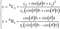
In order to test the general performance of the proposed algorithm and to compare the effectiveness between different road detection algorithms, rules, defined and used in [16], are used in our works. These rules are defined in table 1.

Table 1.

Rules of road detection used in [16]

Contingency table	ground-truth
	non-road	road
non-road road	TN	FN
non-road road	FP	TP
PixelĺCwise measure	Definition
Quality	$g = \frac{TP}{TP + FP + FN}$
Detection rate	$DR = \frac{TP}{TP + FP}$
Detection accuracy	$DA = \frac{TP}{TP + FP}$

About 1000 unstructured road images are randomly selected from the data set to evaluate the performance of the proposed algorithm. The result is shown in table 2. Table 2 shows that the proposed confidence map is very helpful to improve the effectiveness of road detection (the results of both SVM and KNN are also improved when the proposed map is added).

Table 2.

Performance of different road detection algorithms

	g	DA	DR
SVM	0.78±0.12	0.85±0.16	0.90±0.15
KNN	0.79±0.11	0.85±0.14	0.91±0.11
SVM + confidence map	0.85±0.07	0.95±0.05	0.89±0.06
KNN + confidence map	0.86±0.06	0.94±0.05	0.90±0.05
algorithm1 [16]	0.75±0.16	0.92±0.07	0.82±0.19
algorithm2 [16]	0.84±0.23	0.87±0.3	0.90±0.22
SVM + KNN + confidence map	0.86±0.04	0.96±0.02	0.91±0.05

The proposed algorithm is also compared with the state-of-the-art method offered by [16], the performance of the proposed algorithm is outlined as shown in table 2. From the results, it can be derived that our algorithm improves the overall performance of road detection.

Our algorithms were implemented in VC2008 on a PC with i7 process, four cores and four GB memory. The average computational time per image is about 30ms for both of SVM and KNN. The proposed confidence map saved about 30% of the traditional computing time, for these pixels where their corresponding probability are 0% (which means background) or are 100%(which means road surface) need not to compute. The proposed algorithm would cost 50 ms to compute an image. However, parallel computing can be applied to reduce the computing time since all visual cues can be executed separately.

5. Conclusion

Unstructured road detection is a challenging problem due to its unstructured nature. Contextual information is important for unstructured road detection. Road distribution is one of the most important pieces of contextual information. We theoretically analysed the road distribution according to the relationship between camera parameters and vehicle pose. Experiments were designed to verify whether the confidence map is helpful compared with the traditional road detection algorithms. Two traditional road detection algorithms, SVM and KNN, were used in our real-road experiments. A typical lower level feature, named the histogram of RGB values, was used both in SVM and KNN. The results show that the proposed confidence map is very useful in road detection. On this basis, a novel method of combining SVM, KNN and the proposed confidence map under the Bayesian framework was proposed to improve the overall performance of the unstructured road detection. Experiments show that the proposed method is effective and has greatly improved the effectiveness of road detection.

Footnotes

6. Acknowledgements

This work was supported in part by the National Natural Science Foundation of China under grant no. 90820015.

References

DeSouza

G.N.

and Kak

A.C.

. Vision for mobile robot navigation: A survey. Pattern Analysis and Machine Intelligence, IEEE Transactions on, 24 (2):237–267, 2002.

Chapuis

Aufrere

, and Chausse

. Accurate road following and reconstruction by computer vision. Intelligent Transportation Systems, IEEE Transactions on, 3 (4):261–270, 2002.

Alon

Ferencz

, and Shashua

. Off-road path following using region classification and geometric projection constraints. In Computer Vision and Pattern Recognition, 2006 IEEE Computer Society Conference on, volume 1, pages 689–696. IEEE, 2006.

Kong

Audibert

J.Y.

, and Ponce

. General road detection from a single image. Image Processing, IEEE Transactions on, 19 (8):2211–2220, 2010.

Finlayson

G.D.

Hordley

S.D.

, and Drew

M.S.

. On the removal of shadows from images. IEEE Transactions on Pattern Analysis and Machine Intelligence, pages 59–68, 2006.

Alvarez

JMA

and Lopez

A.M.

. Road detection based on illuminant invariance. Intelligent Transportation Systems, IEEE Transactions on, 12 (1):184–193, 2011.

Sotelo

M.A.

Rodriguez

F.J.

Magdalena

Bergasa

L.M.

, and Boquete

. A color vision-based lane tracking system for autonomous driving on unmarked roads. Autonomous Robots, 16 (1):95–116, 2004.

Tan

Hong

Chang

, and Shneier

. Color model-based real-time learning for road following. In Intelligent Transportation Systems Conference, 2006. ITSC'06. IEEE, pages 939–944. IEEE, 2006.

Huang

Y.R.

and Pan

Y.L.

. Fast algorithm for structured and unstructured road detection. In Image and Signal Processing, 2009. CISP'09. 2nd International Congress on, pages 1–5. IEEE, 2009.

10.

Gao

Luo

, and Moli

. Rough set based unstructured road detection through feature learning. In Automation and Logistics, 2007 IEEE International Conference on, pages 101–106. IEEE, 2007.

11.

Foedisch

and Takeuchi

. Adaptive road detection through continuous environment learning. In Information Theory, 2004. ISIT 2004. Proceedings. International Symposium on, pages 16–21. IEEE, 2004.

12.

Wang

, and Zhang

. Color-based road detection in urban traffic scenes. Intelligent Transportation Systems, IEEE Transactions on, 5 (4):309–318, 2004.

13.

Huang

Kong

, and Zheng

. A new method of unstructured road detection based on hsv color space and road features. In Information Acquisition, 2007. ICIA'07. International Conference on, pages 596–601. IEEE, 2007.

14.

Wang

, and Su

Y.T.

. Unstructured road detection using hybrid features. In Machine Learning and Cybernetics, 2009 International Conference on, volume 1, pages 482–486. IEEE, 2009.

15.

Yim

Y.U.

and Oh

S.Y.

. Three-feature based automatic lane detection algorithm (tfalda) for autonomous driving. Intelligent Transportation Systems, IEEE Transactions on, 4 (4):219–225, 2003.

16.

Alvarez

J.M.

Gevers

, and Lopez

A.M.

. 3d scene priors for road detection. In Computer Vision and Pattern Recognition (CVPR), 2010 IEEE Conference on, pages 57–64. IEEE, 2010.

17.

López

Serrat

Cañero

Lumbreras

, and Graf

. Robust lane markings detection and road geometry computation. International Journal of Automotive Technology, 11 (3):395–407, 2010.

18.

Dalal

. Finding people in images and videos. PhD thesis, Institut National Polytechnique de Grenoble-INPG, 2006.

Robust Unstructured Road Detection: The Importance of Contextual Information