Sage Journals: Discover world-class research

Abstract

Data association is critical for Simultaneous Localization and Mapping (SLAM). In a real environment, dynamic obstacles will lead to false data associations which compromise SLAM results. This paper presents a simple and effective data association method for SLAM in dynamic environments. A hybrid approach of data association based on local maps by combining ICNN and JCBB algorithms is used initially. Secondly, we set a judging condition of outlier features in association assumptions and then the static and dynamic features are detected according to spatial and temporal difference. Finally, association assumptions are updated by filtering out the dynamic features. Simulations and experimental results show that this method is feasible.

Keywords

Simultaneous Localization and Mapping Data Association Dynamic Obstacle Outlier

1. Introduction

Simultaneous Localization and Mapping (SLAM) is a fundamental and difficult problem in mobile robotics^[1–2]. It is one of the most important qualifications for mobile robots in realizing autonomy. Data association in SLAM is a process for establishing the correspondence between the sensor measurements (or observations) and map features in order to determine whether they originated from the same physical characteristic in the environment^[2]. It is the prerequisite and basis for state estimation and it influences the real-time performance and accuracy of SLAM. Therefore, data association plays a very important role in SLAM. However, most real world states are dynamic and moving obstacles cause false data associations which compromise the overall quality of the map. The issue of how to eliminate the interference of dynamic obstacles is essential for the SLAM data association problem in dynamic environments.

At present, there are many data association algorithms applied in SLAM and – among them – the most commonly used are Individual Compatibility Nearest Neighbour (ICNN)^[3], Joint Compatibility Branch and Bound (JCBB)^[4] and Multiple Hypothesis Tracking (MHT)^[5]. In addition, Tim Bailey introduced the graph theory into SLAM data association by looking for two complete graphs and the maximum common sub-graph between the observations and the map ^[6]. This method has strong anti-interference capabilities but the problem of searching the largest common sub-graph is difficult. Furthermore, geometric constraints between observations have to be extracted in order to construct the complete graph. Moreover, when the number of the observations increases, the computation will increase significantly. Zhang Sen^[7] converted the SLAM data association to the 0–1 integer programming problem and used multi-dimensional assignment to solve the single frame data association. It is robust but it cannot be applied in real-time. Dirk^[8] proposed a lazy method which needs to calculate the inverse matrix of a large dimension. In other approaches, evolutionary computation, such as the ant colony algorithm, is used in data association^[9]. The ICNN and JCBB algorithms are mostly used in static environments and they are less effective when used directly in dynamic environments. Many researchers applied the MHT algorithm to do data association in a dynamic environment because it can track dynamic targets. To maintain tracking features, the MHT algorithm is of high computational complexity, which hinders the real-time implementation of the SLAM process.

In this paper, in order to take account of real-time and accuracy, we use a simple strategy to achieve the data association in dynamic environments based on the hybrid data association algorithm^[10] and the spatial and temporal difference dynamic features detection method. Initially, we present a hybrid approach of data association based on local maps by combining the ICNN and JCBB algorithms. ICNN is firstly used to do data association in the local map whose arrangement is determined by the preset threshold. In order to overcome the problem of the low reliability of ICNN, error detection in the data association results is necessary. If there are mismatches, JCBB will be used in the local area around the mismatched measurements to correct them. Secondly, we set a judging condition of outlier features and the outlier property of features is used within the spatial and temporal difference to detect dynamic features in association assumptions which are calculated by the above hybrid approach. Finally, the association assumptions are updated by filtering out the dynamic features. We refer to the method as LIJ-STD (Local ICNN-JCBB with Spatial and Temporal Difference).

2. Hybrid Data Association

2.1 Data Association Problem in SLAM

During the process of SLAM, we suppose that there are n features F={F₁, F₂, …, F_n} in a built map and m observations E={E₁, E₂, …, E_m} by the sensors. The data association is to set the relationship between the features and the observations, which can be described as K_t:

K_{t} = {k_{1}, k_{2}, \dots, k_{m}}

(1)

If the ith observation E_i (i=1, 2, …, m) corresponds to the jth map feature F_j (j=1, 2, …, n), then k_i=j (k_i∊K_t). If the ith observation E_i cannot correspond to any features, then k_i=0, which means that the observation E_i may be a new feature or a false observation.

The ith observation at time t denoted z_t,i is given by:

z_{t, i} = h_{t, j} (x_{t | t - 1}) + ω_{t, i}

(2)

where h_t,j () is a non-linear observation function which models the relationship between the system observations and the system state and ω _t,i is a random vector of measurement noise with zero mean and covariance R _t,i. The observation function is linearized around the current estimation by:

h_{t, j} (x_{t | t - 1}) ≅ h_{t, j} ({\hat{x}}_{t | t - 1}) + H_{t, j} (x_{t} - {\hat{x}}_{t | t - 1})

(3)

where the Jacobian $H_{t, j} = {\frac{\partial h_{t, j}}{\partial x_{t | t - 1}} |}_{({\hat{x}}_{t | t - 1})}$ . The distance between the ith observation and the jth map feature can be calculated by the innovation ν _t,ij and innovation covariance S _t,ij:

υ_{t, i j} = z_{t, i} - h_{t, j} ({\hat{x}}_{t | t - 1})

(4)

S_{t, i j} = H_{t, j} P_{t | t - 1} H_{t, j}^{Τ} + R_{t, i}

(5)

The individual compatibility between E_i and F_j can be determined by the Mahalanobis distance with innovation, as follows:

D_{t, i j}^{2} = υ_{t, i j}^{Τ} S_{t, i j}^{- 1} υ_{t, i j} < χ_{d, 1 - α}^{2}

(6)

where d=dim(h_t,j) and 1-α is the desired confidence level (usually set to 95%).

The ICNN selection criterion for a given measurement is to choose that with the smallest distance between the features which falls in the acceptance region according the formula (6). The ICNN algorithm needs do the association test m×n times. Thus, its computation is linear with the map features, O(mn). The ICNN is easy to realize and has low computational complexity, but its antijamming capability is weak. It is only suitable for situations where there are few features or large intervals between the features.

The ICNN algorithm can only guarantee the locality correctly because it does not make overall consideration. That is to say, the individual compatibility cannot be guaranteed to be jointly compatible in forming a consistent hypothesis. In order to ensure the SLAM process consistently, all of the measurements should be jointed so as to find the associated features. The JCBB algorithm considers all of the observations at one frame and determines the association by the Mahalanobis distance of the joint pairs. When the features of the mobile robot working environment are many and near to each other, the JCBB algorithm is working better and is more reliable than the ICNN. However, the JCBB algorithm's computation is exponential in relation to the number of observations. With the environment expanding, its run-time will be significantly increased. Thus, the JCBB algorithm is only fit for a small environment.

2.2 The Hybrid Data Association Approach-LIJ

The ICNN and JCBB approaches have their own advantages and disadvantages. We consider making use of their advantages by combining them together. For the sake of time performance, the hybrid approach is mainly based on the real-time ICNN algorithm. Then, in order to improve the accuracy, JCBB is only used locally in order to correct the wrong association pairs in the ICNN results after checking them out. In order to reduce the computational load of JCBB and reduce the time complexity of the hybrid approach, all of the data association processing is done with local maps.

The hybrid data association algorithm LIJ mainly employs the following steps:

Step 1: ICNN data association based on local maps

In the built global map, we establish a circular local map in which there are features which are most likely to match the current observations at time t. In order to cover all of the possible features, the circle's centre is set as the location of the mobile robot and the radius as r:

\sqrt{{(x_{j} - x_{r})}^{2} + {(y_{j} - y_{r})}^{2}} < r

(7)

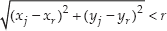
Where (x_r, y_r) and (x_j, y_j) are the positions of the mobile robot and the feature F_j in the global coordinate system, respectively.

The ICNN algorithm is used in the circular local map and gets the association assumption K_t' ={k₁, k₂, …, k_m}.

Step 2: Judgment as to whether there are association errors or not. If yes, then go to Step3, otherwise go to Step4.

Here, we use a general hypothesis: different observations originate from different map features, and a map feature has only one matching observation ^[4,7]. According to the general hypothesis, all of the Kt elements should have different values indexing different features except for the zero valuewhich represents a failure to find the matching feature or a false observation. Therefore, we build a criterion to judge the wrong association pairs: if K_t has elements with the same non-zero value, these elements are wrongly matching pairs.

Step 3: Modification by the JCBB algorithm

(1) Find the observation E_a which should be re-associated.

As JCBB computational complexity increases exponentially with the number of observations, not all of the observations have to be re-associated but rather only those around the wrongly matched map features. Firstly, find out the non-zero element kc (c∊[1, m]) of the same value in Kt'. We can get the map features F_b (b=k_c, k_c∊[1, n]) which have been wrongly matched. Secondly, find out the observation E_a (a∊[1, m]) around the feature F_b by satisfying a threshold d:

\sqrt{{(x_{E_{a}} - x_{F_{b}})}^{2} + {(y_{E_{a}} - y_{F_{b}})}^{2}} < d

(8)

where (x_Ea, y_Ea) and (x_Fb, y_Fb) are the positions of the observation E_a and the feature F_b in the global coordinate system, respectively. The threshold d is an important factor which influences the number of the re-associated observations. If the threshold is set too high, it is not helpful to improving the real-time performance. Otherwise, too small a setting will reduce the accuracy. This has been proven in our experiment.

(2) Calculate the data association between the features F_j in the circular local map and the observations E_a by the JCBB algorithm. The result is used to modify K_t' of Step1.

Step 4: Getting the association result K_t = K_t'. The data association ends at time t.

As can be seen from above, LIJ needs more steps than ICNN to find any wrongly matching pairs; however, the compatibility between the observations and the map features is only calculated in the local map. Thus, when features are sparse, LIJ's computation complexity becomes almost the same as ICNN's. However, as the environment becomes more complex, wrongly matching pairs increase. LIJ's running time increases by using JCBB to correct mistakes. Because the calculations are all done with local maps, LIJ still gives a good time performance.

3. Dynamic Obstacle Detection and Processing Strategy

3.1 Outlier Feature

In dynamic environments, static obstacles and dynamic obstacles need to be identified effectively in the data association. Only static obstacles are used in the SLAM process and dynamic ones are filtered out to ensure the accuracy of the SLAM results. In this paper, we detect dynamic obstacles by the spatial and temporal difference, which is similar to the map differential method. The feature points in the same position or else in the range of a certain threshold space at different times are considered as static obstacles; otherwise they are treated as dynamic obstacles. When the speed of dynamic obstacles is slow, there will be some dynamic obstacles in the association assumptions. The false associations with the dynamic obstacles cannot be effectively detected using the spatial and temporal difference method alone. Thus, we combine with the outlier property of the feature points to detect them.

The movement properties of dynamic and static obstacles are obviously different. Here, we use the Mahalanobis distance between the two corresponding feature points to detect the outlier property. Equations (4), (5) and (6) show that the deviation of the adjacent time observations from the same sensor to the static obstacles is small; as such, the Mahalanobis distances of their matching pairs tend to be more consistent. Under normal circumstances, the matching pairs gotten by the hybrid data association algorithm are mostly static obstacles. If the Mahalanobis distance between the two observations of a matching pair is very different from the other pairs, we can judge that the feature corresponding to the matching pair is dynamic. Based on experiments, the outliers are defined by the Mahalanobis distance as:

{D_{t} | D_{t} < 0.5 \cdot med (D_{t}) | | D_{t} > 1.5 \cdot med (D_{t})}

(9)

where the med (D_t) is the mean value of the Mahalanobis distances for all matching pairs in the association assumptions.

In extreme cases, there are more dynamic features than static ones in the association assumptions and thus using (9) to find the outliers will lead to misjudgements. In addition, because of uncertainties due to the environment and sensor observations – such as sensor misreading – there will be a large error in comparing the adjacent spatial and temporal differences.

In this paper, we set the dynamic and static attribute of the jth map feature F_j at time t as flag_t, _j , and flag_t, _j =1,-1,0 which represent that the feature F_j is static, dynamic and unknown respectively. “0” is a transitional state that temporarily cannot be determined as a static or a dynamic feature. The transitional state enhances the judgment reliability because it means that any feature's dynamic and static attribute is confirmed by at least 2 determination steps. Dynamic features will be filtered out and static and unknown features are used for the state estimation in SLAM. The unknown features will give more environmental and historical information in SLAM.

At the current time, the dynamic and static properties of the new features are set to 0 and there are four cases to update the old features in the map:

If the feature on the map has the corresponding observation at the current time and it is identified as an outlier, its static and dynamic property will be changed to “0” from “1” or to “-1” from “0”;

If the feature on the map has the corresponding observation at the current time and it is identified as not being an outlier, its static and dynamic property will be set to “1”;

If the feature on the map is in the observation range of the sensor at the current time and does not have the corresponding observation, its static and dynamic property will be changed to “0” from “1” or to “-1” from “0”;

If the feature on the map is not in the observation range of the sensor at the current time, its static and dynamic property will remain unchanged.

The updating strategies of the static and dynamic properties are shown in Table 1.

Table 1.

The updating strategies of the feature F_j's static and dynamic properties

flag_t _-1,f	Is F_j in the range of the sensor at time t?	Does F_j have the corresponding observation?	Is F_j an outlier?	flag_t, _j
1	yes	yes	yes	0
0	yes	yes	yes	−1
1	yes	yes	no	1
0	yes	yes	no	1
1	yes	no	/	0
0	yes	no	/	−1
1	no	/	/	1
0	no	/	/	0

3.2 Dynamic Obstacle Processing in Data Association

The processing strategy of dynamic obstacles in the SLAM data association follows these steps:

Step 1: Obtain association assumptions by the hybrid data association method LIJ with the observations and the map features of which static and dynamic properties are “0” or “1”. The observations which are not associated with map features are considered as new features and their static and dynamic properties are set to “0”.

Step 2: Calculate the mean value of the Mahalanobis distances for all matching pairs in the association assumptions and determine whether the pairs are outliers or not by (9). If yes, the observation in the outlier pair is considered as a new feature and the map feature in the outlier pair is considered as not finding any correspondence at that time. Both of them are set with their static and dynamic properties at “0”. If no, the observation and the map feature in the matching pair are indicating the same object and their static and dynamic properties are set to “1”.

Step 3: Determine whether the map features in the observation range. If yes, the features are dynamic and their static and dynamic properties are set from “1” to “0” or from “0” to “-1”. If no, their static and dynamic properties remain unchanged.

Step 4: The features whose static and dynamic properties are “0” or “1” are added to the map and others with “-1” are filtered out.

4. Simulations and Experiments

In order to validate the idea presented in this paper, we test it in an artificial environment and a real outdoor environment.

4.1 Simulation Results

The simulation environment is a 12 meters by 14 meters region – as shown in Figure 2 – in which we pre-set the vehicle's trajectory as an octagon with a dashed line and randomly distribute 100 static landmarks with circles and 10 different dynamic obstacles whose trajectories are marked as irregular curves. In the simulation, the vehicle moves at a linear velocity of 0.3125m/s and the sensor range is 0–3.5m and −90°-+90° while sensing period 1s. Here, the threshold r is set to 4m and d is set to 0.5m.

Figure 1.

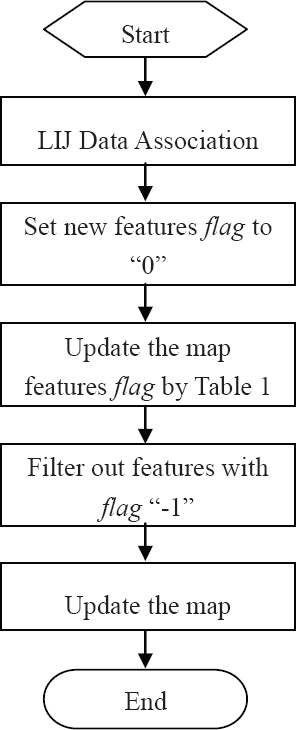
Flowchart of the dynamic obstacle processing strategy in data association

Figure 2.

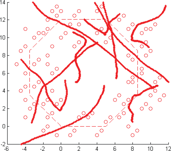
Simulation environment

We apply the LIJ-STD and LIJ data association algorithm to perform the SLAM process. The simulation's experimental results are shown as Fig. 3, in which the blue curve consisting of a series of triangles is the vehicle's trajectory estimation and “+” denotes the landmarks' estimations. From the simulation results, we can see that the estimations of the vehicle trajectory and the landmarks have a larger deviation because of the dynamic obstacles' interference. However, after dealing with the dynamic obstacles by the LIJ-STD algorithm proposed in this paper, we can get a high accurate SLAM result and a high correct rate for the data association. Figure (b) indicates that this method can effectively reduce the dynamic obstacles' interference and, after filtering out dynamic obstacles, the SLAM process builds a map which basically contains only static landmarks. From Figure (c) and Figure (d), we can see that the correct association rate of the LIJ-STD algorithm is higher than that for the LIJ algorithm.

Figure 3.

Simulation results

4.2 Real Outdoor Environment

The experimental test in a real outdoor is implemented by the autonomous vehicle developed by Intelligent Lab at Central South University, as shown in Figure 4. It is equipped with a tightly GPS/INS integrated system XW-ADU5630^[11] providing the measurement of the vehicle's position and a laser SICK LMS291 which is an external sensor for sensing the environment. The GPS/INS system and the laser range sensor are combined together to estimate the vehicle's trajectory by a particle filter and to build up the map at the same time. For simplicity, the obvious point-like features including pedestrians, tree trunks, vehicles and the building's convex points, are used as landmarks to build up the map and to do data association in SLAM.

Figure 4.

Experimental Vehicle

The experiment's route in the Tiedao Campus of Central South University and the raw data are shown in Figure 5, in which the yellow curve represents the vehicle's route, the start and end of the route are indicated by red dots, the red curve is GPS/INS system data which is used as vehicle's true trajectory and the black points are the raw data from the laser. It is an outdoor, large-scale and dynamic environment in which there are cars, pedestrians and other dynamic obstacles. This information will serve as a reference to the SLAM results.

Figure 5.

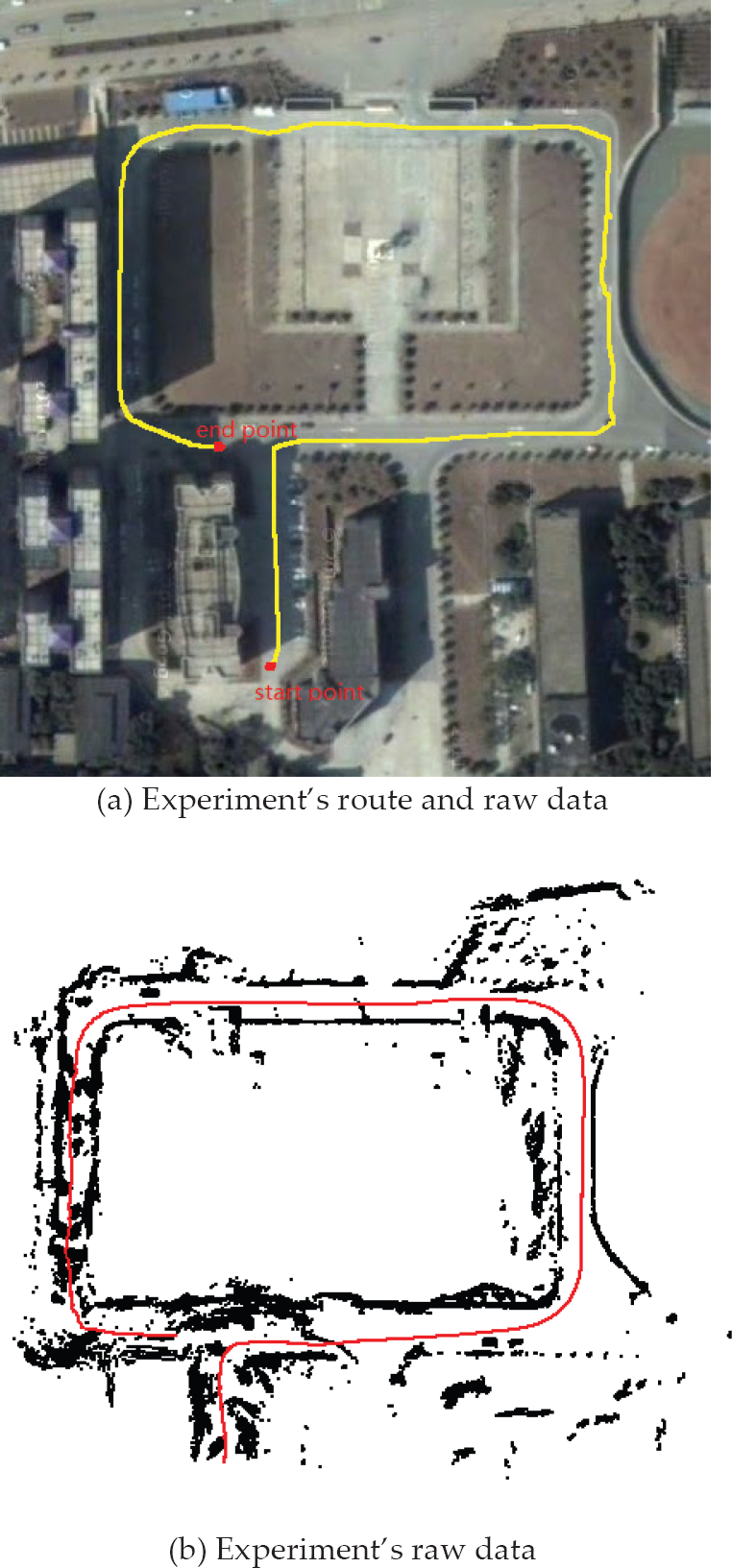
Experiment's route and raw data

The experimental results are shown in Figure 6, in which the blue dotted line is the vehicle's trajectory estimation and the green dot is the estimation of the point-like features which are used to do the data association. Next, we have calculated the vehicle position errors relative to the GPS/INS system. The mean and standard deviation of the errors are 9.72m and 4.85m with the LIJ algorithm and 4.25m and 2.29m with the LIJ-STD algorithm. By comparison, between the SLAM results with the LIJ algorithm and with the LIJ-STD algorithm, we can see that, in a dynamic environment and with the LIJ-STD algorithm, the vehicle trajectory estimation is more consistent with GPS by dealing with dynamic obstacles, and the SLAM results have been improved because the correct rate of the data association is enhanced, which proves the effectiveness of the method.

Figure 6.

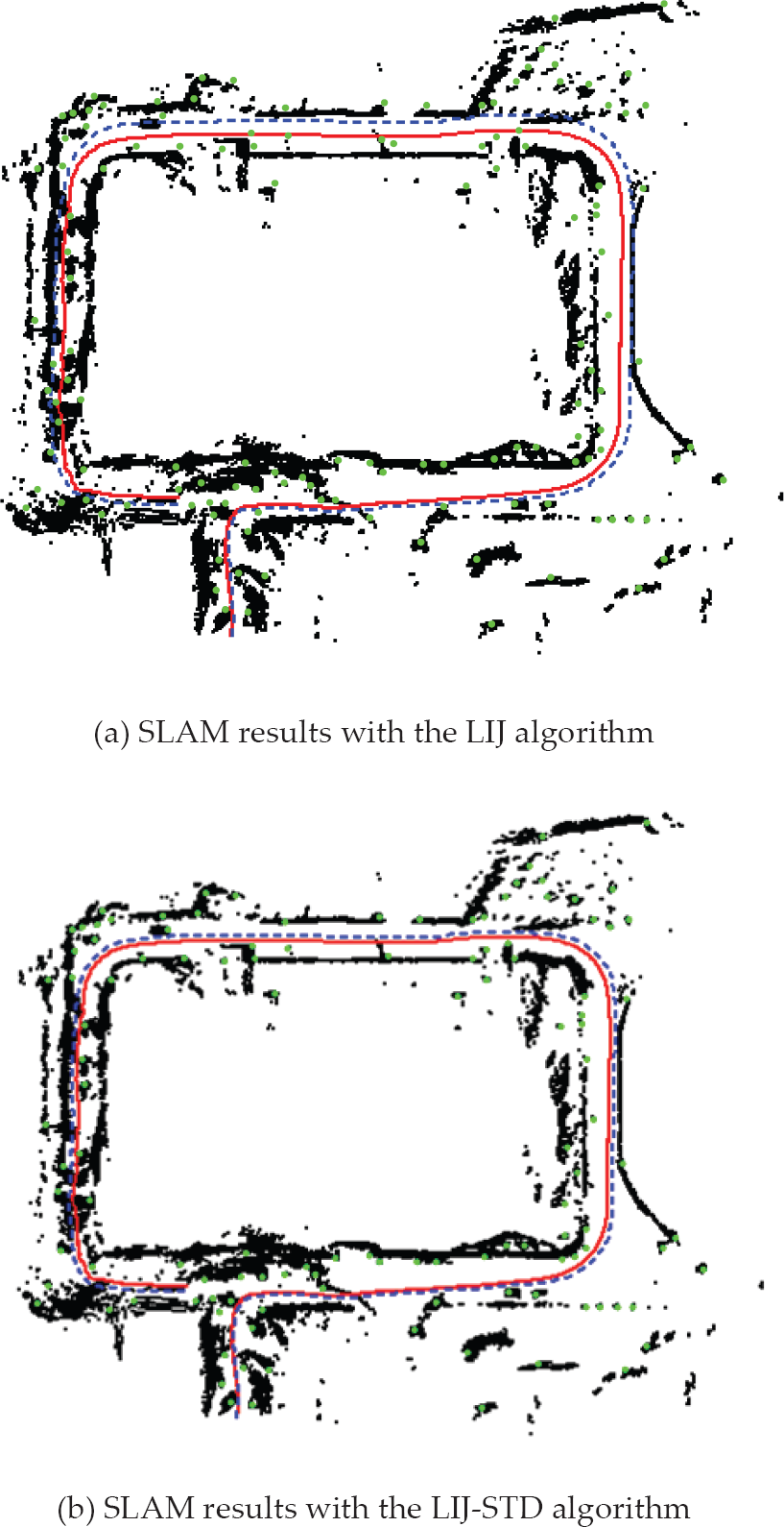
Experiment Results

5. Conclusions

In this paper, the issue of how to deal with dynamic obstacles based on a hybrid data association approach with the spatial and temporal difference in the process of data association was discussed. We combined the classic data association algorithms ICNN and JCBB with local maps, which gave good time performance and accuracy. In addition, we built a judging condition to detect outlier features in the association assumptions. The outlier property of the features was used in the spatial and temporal difference to determine whether the features were static or dynamic. Simulations and the vehicle's experimental results in a realistic outdoor environment showed that this method can eliminate dynamic obstacles' interference and that it has a high correct data association rate and helps with performing SLAM successfully.

Footnotes

6. Acknowledgments

The research work is jointly supported by the National Natural Science Foundation of China under Grant 90820302 and Hunan Province Natural Science Foundation of China under Grant 12JJ3064

References

Durrant-Whyte

Bailey

, “Simultaneous localization and mapping: Part I,” IEEE Robotics and Automation Magazine, Vol.13, No.2, pp. 99–110, 2006.

Bailey

Durrant-Whyte

, “Simultaneous localization and mapping: Part II,” IEEE Robotics and Automation Magazine, Vol.13, No.3, pp. 108–117, 2006.

Guivant

J. E.

Nebot

E. M.

, “Optimization of the simultaneous localization and map-building algorithm for real-time implementation,” IEEE Transactions on Robotics and Automation, Vol.17, No.3, pp. 242–257, 2001.

Neira

Tardos

J. D.

, “Data association in stochastic mapping using the joint compatibility test,” IEEE Transactions on Robotics and Automation, Vol.17, No.6, pp. 890–897, 2001.

Davey

S. J.

, “Simultaneous localization and map building using the probabilistic multi-hypothesis tracker,” IEEE Transactions on Robotics, Vol.23, No.2, pp. 271–280, 2007.

Bailey

Nebot

E. M.

Rosenblatt

J. K.

, “Data association for mobile robot navigation: A graph theoretic approach,” IEEE International Conference on Robotics and Automation. San Francisco, USA, pp. 2512–2517, 2000.

Zhang

Xie

Adams

, “An efficient data association approach to simultaneous localization and map building,” IEEE International Conference on Robotics and Automation. New Orleans, USA, pp. 854–859, 2004.

Hahnel

Thrun

Wegbreit

, “Towards lazy data association in SLAM,” Robotics Research, No. 15, pp. 421–431, 2005.

Zeng

Zhang

, “Data association method of SLAM based on ant colony algorithm,” Journal of Computer Applications, Vol. 29, No. 1, pp. 136–148, 2009.

10.

Chen

Cai

Zou

, “A Hybrid Data Association Approach for Mobile Robot SLAM,” International Conference on Control, Automation and Systems. Kintex, Korea, pp. 1900–1903, 2010.

11.

STARNETO TECHNOLOGY DEVELOPMENT CORPORATION. Manual of XW-ADU5630 GPS/INS integrated system [EB/OL]. [2010-05-27]. http://www.3dgps.com.cn/proshow.asp?ArticleID=278.

A Hybrid Data Association Approach for SLAM in Dynamic Environments

Abstract

Keywords

1. Introduction

2. Hybrid Data Association

2.1 Data Association Problem in SLAM

2.2 The Hybrid Data Association Approach-LIJ

3. Dynamic Obstacle Detection and Processing Strategy

3.1 Outlier Feature

3.2 Dynamic Obstacle Processing in Data Association

4. Simulations and Experiments

4.1 Simulation Results

4.2 Real Outdoor Environment

5. Conclusions

Footnotes

6. Acknowledgments

References