
Abstract
For the local path-planning of multi-robots, a decentralized method is presented where each robot plans its own path in the following steps for each iteration. Firstly, an optimal way representative point (OWRpoint) is obtained for guiding the robot to move along a shorter path. Then, the robot moves a step under the control of its own motion controller, which is designed based on artificial moments. In the motion controller, attractive and repulsive moments are used to move robots closer to their OWRpoints and away from obstacles, while coordinated moments are used to resolve the conflicts between robots. Two simulations are given to test the method and the results indicate that the method is valuable as it meets the requirements of the real-time property while optimizing the performance measure of each robot: namely, the path travelled to reach the robot's target.
1. Introduction
As remarked upon in [1], there has been a growing interest in multi-robot systems in recent years and motion planning is of primary importance in the design of multi-robot systems. This paper focuses on a version of the problem that concerns the path-planning of multiple autonomous mobile robots. The environment is populated with various obstacles. No robot has a priori knowledge about the environment or other robots. The objective is to simultaneously bring each robot from an initial position to an independent target. In addition to ensuring collision avoidance, each robot has a performance measure - the path travelled to reach its target - to be optimized.
As no robot has a priori knowledge, the problem is a form of local or online path-planning for multi-robots [2]. As individual performance measures are not combined into a single scalar criterion, the problem differs from that discussed in [3], [4], where the criterion is to minimize the time taken by the last robot to reach its target. As remarked upon in [5], when individual performance measures are combined, certain information about potential solutions and alternatives are lost. For example, the degree of sacrifice that each robot makes in order to avoid other robots is not usually taken into account.
Many approaches have been developed for multi-robot path-planning, which are often categorized as centralized or decentralized [5], [6], [7]. With centralized methods, a central planner designs the motion plan for all of the robots based on full knowledge about the environment. Decentralized approaches require that each robot plans its own path based only on the locally available information - e.g., the positions of neighbouring robots - so that it requires less computational resources and also ensures the scalability of the system.
Obviously, only decentralized approaches can be used for the local path-planning of multi-robots as no robot has full knowledge about the environment or other robots.
In [2], [8], [9], a decentralized method based on evolutionary algorithms (EAs) or differential evolution algorithms is discussed, where n EAs are used for n robots and the i-th EA determines the next position for the i-th robot during each iteration, satisfying the necessary constraints associated with that robot and certain cooperation objectives related with the others. In [10], [11], prioritized planning is discussed, which works as follows. First, priorities are assigned to the robots. Then, in order of decreasing priority, the robots are picked. For each picked robot, a path is planned, avoiding collisions with obstacles as well as with the previously picked robots. The drawback of the two methods is the requirement of a considerable amount of communication.
In recent years, the artificial potential field (APF) method is extended to multi-robot path-planning [12], [13]. Here, a repulsive potential field to force a robot away from obstacles or other robots and an attractive field to drive the robot close to a target are employed to generate a force. The force equals the negative gradient of the total potentials and makes the robot move from a position with higher potentials to one with lower potentials. This method requires only a simple calculation and no pre-processing of the environment, but powerful results and elegance of output are generated in a short time [12], [14]. However, this method suffers from many problems [12], [13], [14], [15], such as the “local minimum” problem. When it is used for multi-robot path-planning, coordination between robots is difficult to obtain through the pure APF method as robots cannot be regarded as simply obstacles, and as such some other techniques, such as priorities, have to be used [12], [13].
The configuration space method [12], [16], [17] and the free space method [16], [18], [19] are the methods directly used not only for multi-robot path-planning but also as the basis of other methods, such as the probabilistic roadmap method [20]. In the configuration space, the original problem of planning the motion of a robot through a space of obstacles is transformed into an equivalent - but simpler - problem of planning the motion of a point through a space of enlarged configuration space obstacles or pseudo-obstacles. The free space method is to search the free space directly without first transforming the problem into a configuration space. A representation of a free space can be obtained using generalized Voronoi diagrams [16], a tangent graph [18] or a visibility graph [19]. The drawback of the two techniques is that in local path-planning the configuration space or the free space is frequently required to be recomputed, considering the safe distance and the sizes of the robots. Again, a great deal of computation is needed.
In fact, and to the best of our knowledge, although many algorithms have been developed for the local path-planning of multi-robots, very few can not only meet the requirements of a real-time property but also optimize each robot's performance measure well. Activated by the limitation noted above, a decentralized method is proposed for multi-robot path-planning, which is an extension of the artificial moment method for multi-robot formation control [21], [22].
In the proposed method, each robot which has not reached its target or which is required to cooperate with other robots uses a path planner, which works as follows. At each sampling time, an optimal way representative point (OWRpoint), which can guide the robot in moving along a shorter path, is obtained firstly, ignoring the presence of other robots. Then, a motion controller based on artificial moments causes the robot to move a step to the next position. The above process is repeated until the task is fulfilled. The proposed method is valuable as it not only meets the requirements of a real-time property, but it also optimizes the independent performance measure of each robot well.
The rest of this paper is organized as follows. In section 2, the problem under discussion is formulated and some concepts are defined. In section 3, the techniques and algorithms for computing OWRpoints are presented. In section 4, a motion controller based on artificial moments is designed. In section 5, the algorithm for the path-planning is given. Several simulations are given and analysed in section 6 and certain conclusions are drawn in section 7.
2. Problem formulation and basic definitions
2.1 Problem Formulation
This paper focuses on the path-planning of multi-robots in a bounded planar environment which is populated with static polygonal obstacles.
A robot model is a square, as shown in Fig. 1, which has a principal motion direction line (PMDline) such as that in [21], [22] and two coordinated segments. The PMDline of a robot is a ray starting from the robot's position (the centre) and can indicate the robot's posture or motion direction.

Associated model
A target model is a static point with a PMDline, as shown in Fig. 1. The PMDline of a target indicates the target's posture.
We rotate a directed line (ray, directed segment) around its start-point until its direction is the same as that of the X-axis of the global coordinate system. As such, the angle formed by the rotation is the direction angle of the line if the angle's absolute value is not larger than π. Assume that β i and β i are the direction angles of directed lines li and lj and that n is an integer and function:

Then, the angle β=agl(βi-βj) is the angle from li to lj.
For convenience, certain notations which will be used throughout this paper are listed as follows.
DR, SR: the side length and longest step length of a robot;
DV: the valid radius of a robot's sensor;
DS: a constant which is larger than 2SR+DR and is associated with the robots' safeties;
DM: a positive constant less than DS;
δθ2: a constant which is less than π/2 but not π/4;
δθ1: a positive constant far less than δθ2;
λ1, λ2 two constants satisfying 0 <λ1<λ2<1;
λπ: a constant whose value is π/DS;
Ri, Ti: the i-th robot and the target of the i-th robot;
β Ri , β Ti : the PMDline direction angles of Ri and Ti;
PRi: the position (the centre) of Ri;
(xRi, yRi) T : the position coordinates of R;
PMi: a point on Ri's PMDline with a distance DM from PRi;
(xTi, yTi) T : the position coordinates of Ti;
A1 A2: the line segment with end points A1 and A2;
DS(A1, A2): the directed line segment from A1 to A2;
β(A1, A2): the direction angle of DS(A1, A2);
RL(A1, A2): a ray starting from A1 and passing through A2;
| W|: the length of a continuous curve W;
∂(W,-A1,…,-An): points on W except for points A1, …, An;
∂(RL(A1, A2), -A1 A2): points on RL(A1, A2) except for those
on A1A2; A1A2… An: a polyline with vertices A1, A2, …, An. For an arbitrary variable V, V(k) denotes its value at time tk and V denotes it at the present.
A robot's coordinated segments are two directed segments whose lengths are DS+DR, the start-points are the robot's position while angles to the PMDline are ±π, as shown in the model of Ri in Figure 1. The coordinated segments are important in resolving the conflicts between robots.
The robot sensors are omni-directional. For a point F, only when PRiF does not pass through any obstacle (including robots) and | PRiF | ≤ DV, can F be detected by Ri. For two robots, only when the segment between their positions does not pass through any obstacle and is shorter than DV can they be detected and their positions and PMDlines be known by each other.
For example, in Figure 1 only R and its PMDline, as well as the points within the region with a grey colour or on the boundaries of the region, can be detected by R at present. The point A1 can be detected by R at Ri 's initial position but cannot be detected at Ri 's current position.
As it is important to reduce the communication required between robots to the absolute minimum (otherwise realtime dynamic planning will not be possible) there is no explicit communication between robots in this paper. That is to say, a robot has no knowledge about other robots until it detects them and, then, it knows - and only knows - their positions and PMDlines at the present. A robot also has no a priori knowledge about its workspace.
2.2 Basic Definitions
For example, in Figure 1, A1A2A3A4 is a knowledge obstacle wall of Ri and A1, A2, A3, A4 are its vertices; A1A2 A3A4A5 is not so because some points on it, such as A5, have never been detected by Ri.
Each robot will memorize and update all of its knowledge obstacle walls.
For example, in Figure 1, A1A2A3A4 is a block wall of R; PRiA 4 Ti and PRiA2A1A3Ti are free block-wall ways of Ri, but PRiA2A3Ti is not because it is blocked by A1A2A3A4.
The shortest free block-wall way is important as a shorter, feasible way can be easily obtained through it. Furthermore, compared with the shortest feasible way obtained by such methods as the tangent graph method and the configuration space method, the shortest free block-wall way is easier to obtain as there is no requirement to consider the safe distance of robots and no requirement to pre-process the environment.
As obstacles are all polygons, the shortest free block-wall way of R must be a polyline. Assume it is PRiA1A2,…,AnTi; then, the first vertex A1 but not the full way is needed to be obtained for guiding Ri to move. The reasons for this are that, as the shortest free block-wall way of Ri at present is often significantly different from that at the next in local path-planning, it is effective only at the present.
Moreover, at the current time, A1 has the same effect as the full way for optimizing Ri 's path but is easier to obtain and requires less memory.
For example, when PRiTi is not blocked by any knowledge obstacle wall of Ri, Ti is the OWRpointi.
For example, in Figure 1, Ri and Rj are coordinated companions of each other.
Obviously, a dangerous wall representative point of Ri is the point that is the shortest distance from PRi in a local region of a dangerous knowledge obstacle wall. Accordingly, for Ri, several such points may exist on the same knowledge obstacle wall, which can prevent Ri from colliding with one side while avoiding another side of the wall.
For example, in Figure 2, RL(PRi, A4) is a single-direction tangent from PRi to Σ and A4 is the tangent point. RL(PRi, A1) is a close tangent from PRi to Σ1 (Σ2 and Σ1 are merged into one wall by an artificial obstacle segment V3V4) and A1 and F1 are the tangent and the close point respectively. RL(A1, A2), RL(A2, A3) are close tangents of R.

Single-direction and close tangents, artificial obstacle segments
3. Method for OWRpoints
In this section, a method is presented to determine a series of OWRpoints which guide each robot to move along a shorter path. The first step of this method is to set artificial obstacle segments according to the rules given as follows until no such segments can be set. Since such segments can block these ways onto which the OWRpoints are not suitably placed, the computation of the OWRpoints is decreased by setting such segments.
3.1 Rules for Setting Artificial Obstacle Segments
There are two types of artificial obstacle segments, namely narrow-types (N-type) and back-types (B-type).
The rule for N-type artificial obstacle segments is as follows. For two points A1 and A2 on knowledge obstacle walls of Ri, if |A1A2| is less than 2DS and a free block-wall way of Ri passes through A1A2 once and once only, then A1A2 can be set as an N-type artificial obstacle segment. For example, in Figure 2, V3V4 is an N-type artificial obstacle segment of Ri.
N-type artificial obstacle segments are used to prevent a robot from walking along ways narrower than 2DS, as if two robots encounter each other in a way that is narrower than 2DS, they may be blocked by each other such that their convergence is lost. As remarked upon in [6], the loss of convergence in this case is not a matter of a good or a bad algorithm - it is due to the decentralized control model.
The rules for B-type artificial obstacle segments are as follows. For Ri, assume Σ1 and Σ2 are two different knowledge obstacle walls and that Σ1 blocks PRiTi. 1) If Σ2 also blocks PRiTi, then A1A2 can be set as such a segment, where A1 and A2 are the intersections of PRiTi with Σ1 and Σ2 respectively. 2) Assume that A1 is the tangent point of a close or single-direction tangent from PRi to Σ1. If Σ2 blocks PRiA1 and A2 is an intersection of PRiA1 with Σ2, then A1A2 can be set as such a segment.
For example, V1V2 in Figure 2 is a B-type artificial obstacle segment of Ri. Obviously, for Ri, if A1A2 can be set as a B-type artificial obstacle segment at present, then no point (except for A1 and A2) on A1A2 can be detected at present; however, A1A2 may have been detected at some previous time because A1 and A2 are all on knowledge obstacle walls. That is to say, Ri has moved from a position with a shorter distance from A1A2 to the current one with a longer distance. Thus, walking towards A1A2 will result in walking backwards, which is the reason for calling such segments B-type artificial obstacle segments.
Setting B-type artificial obstacle segments has two main benefits. One is to guarantee the global convergence to a certain extent by preventing a robot from walking backwards. The second is to decrease the total number of knowledge obstacle walls of a robot by merging two different walls into one wall.
Artificial obstacle segments are dealt with as a part of knowledge obstacle walls in general. However, if a closed curve by which Ri and Ti are separated is formed by a knowledge obstacle wall of Ri, then all B-type artificial obstacle segments on the wall will be removed.
3.2 Algorithm to Determine OWRpoints
For Ri, after setting artificial obstacle segments, an OWRpoint will be obtained, which is based on the following conclusions.
1: Let A0 =PRi, Al = A1 and, then, go to step 2.
2: If AlTi is not blocked by Σ, then stop. Otherwise, go to step 3.
3: If a close tangent from Al to Σ exists, then the tangent point is Al+1. Let Al = Al+1 and then return to step 2. Otherwise, go to step 4.
4: If Al =A1, then A2 is the tangent point of the single-direction tangent from A1 to Σ such that A0A2* is blocked by Σ, where A2* is a point on A1A2 and close to A1. Otherwise, Al +1 is the tangent point of the single-direction tangent from Al to Σ that shares no point with RL(Al-2, Al -1). Let Al = Al +1; then return to step 2.
Based on previous discussion, an algorithm for the OWRpointi at present is given as follows.
1: If Ri has no block wall, then Ti is the OWRpointi; otherwise, go to step 2.
2: Assume that Σ is a block wall of Ri. If a close tangent from PRi to Σ exists, then its tangent point is the OWRpointi; otherwise, go to step 3.
3: Obtain the tangent points A1 and Q1 of the two single-direction tangents from PRi to Σ.
4: Obtain FBWA1 and FBWQ1 respectively.
5: Substitute PRi in FBWA1 and FBWQ1 with PMi, such that another two ways represented with FBWA1* and
FBWQ1* are obtained.
6: If |FBWA1*|<|FBWQ1*|, then A1 is the OWRpointi; otherwise Q1 is.
For algorithm 2, the necessary computation in the worst case is to compute |FBWA1| and |FBWQ1| using algorithm 1. Assume that m is the vertex number of the knowledge obstacle wall of Ri with most vertices; then, the computational complexity of algorithm 2 is O(2m) as the number of vertices on FBWA1/FBWQ1 cannot be more than m.
4. Motion controller based on artificial moments
A motion controller based on artificial moments is designed in this section, which is an extension of the artificial moment method for multi-robot formation control [21], [22]. Its basic idea is that at each sampling time Ri may be influenced by three types of artificial moments - that is, the attractive moment by the OWRpointi, the repulsive moments by obstacles and the coordinated moments by other robots. The gradient of each artificial moment generates an expected vector for Ri to change position and the PMDline so that the moment can increase as quickly as possible. Additionally, Ri has a motion vector along its PMDline which is not in general determined by artificial moments. The total vector determines the next position and the PMDline direction of Ri and, afterwards, the above process is repeated until the task is fulfilled.
Obviously, the artificial moment method is similar to the APF method in some aspects. Therefore, they have shared advantages. However, there are certain important differences between them.
One of these is that in the artificial moment method each robot has a motion vector along its PMDline which is nearly uninfluenced by artificial moments. Let (Sxi(k+1), Syi(k+1)) T represent the expected vector of Ri along its PMDline in (tk, tk+1]. If the OWRpointi at the current time tk is Ti and the distance from PRi to Ti is not larger than DS, then (Sxi (k+1), Syi(k+1)) T =(0, 0) T ; otherwise:
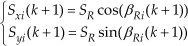
where β Ri (k+1) is Ri's PMDline's direction angle in (tk, tk+1].
The motion vector (Sxi (k+1), Syi(k+1)) T causes Ri to have a high moving speed even if the total moment's gradient is zero and, as such, it is difficult for Ri to be trapped even in complicated environments.
A second difference is that a unique robot model is used in the artificial moment method, where each robot has a PMDline and two coordinated segments. According to the robot model, a coordinated moment - which can resolve the conflicts between robots (almost) optimally - is designed as follows.
4.1 Coordinated Moments
Each coordinated companion of Ri will - and only such robots can - impose a coordinated moment on Ri so that the conflict between them can be solved.
Assume that Rj is a coordinated companion of Ri and that CM(k) is the coordinated moment generated by Rj at the current time tk. The function cmt(x) is defined as (3) and its derivative dcmt(x) as (4):


When |agl(β Ri -β(PRi, PRj))|<δθ2 and |agl(β Ri -β(PRj, PRi))|<δθ2 (the case where Ri and R have a marked trend to move towards each other), CM(k) is required to cause Ri to move to a side of R so that Ri can bypass R and so that no collision occurs between them. Furthermore, according to the PMDlines of Ri and R at present, it can be concluded that the two robots are moving towards PMi and PMj respectively. Accordingly, CM(k) is required to make Ri move towards a position that is away from PMj but close to PMi so that their influence upon the motion of each other can be minimized.
Let M represent the end-point of the directed segment whose start-point is PRj; the direction angle is the same as that of DS(PMj, PMi) and the length is DS+ DR (as shown in Figure 1); (xM, yM) T represents the coordinates of M. As such, M is an ideal point towards which Ri moves as M satisfies all of the requirements mentioned above. Thus, CM(k) is designed as (5) in this case:
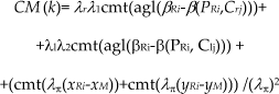
where C lj and C rj are the end-points of the left and right coordinated segment of R j respectively; λ r =D S /(|P Ri C rj |+ D S ) and λ l = D S /(|P Ri C lj |+ D S ).
In (5), only when PRi is at M does CM (k) have the potential to be the greatest. Thus, CM (k) will cause Ri to move towards M. However, when PMiPMj is parallel to PRiPRj, Ri ‘s motion towards M and Rj 's similar motion will lead the two robots to move in parallel and, then, a deadlock arises. To avoid the deadlock situation, the first term, λ,λ1cmt[agl(β Ri (k)-β(PRi, Crj))] and the second, λ1,λ2cmt[agl(β Ri (k)- β(PRi, Clj))] are designed. The first term is to make Ri 's PMDline point to Crj, as the term will be the greatest when Ri 's PMDline points to Crj; the second is to make Ri 's PMDline point to Clj for the same reasons. As λ1< λ2, the influences of the two terms are not the same in general. As a result, PMiPMj cannot be parallel to PRiPRj at next time, even if PMiPMj is parallel to PRiPRj at present. Accordingly, the deadlock situation is avoided.
The coefficient λ x = DS/(|PRiCrj| + DS) will increase with the decrease of |PRiCrj | since the smaller that |PRiCrj | is, the greater the first term is expected to be so that Ri's PMDline can point to Crj and R can move towards Crj. For the same reason, the coefficient λ 1 = DS/(|PRiCrj| + DS) will increase with the decrease of | PRiClj |.
When |agl(β Ri -β(PRi, PRj))|≥δθ2 or |agl(β Rj -β(PRj, PRi))|≥δθ2 (the case where Ri and Rj have no marked trend to move towards each other), CM(k) is only required to ensure that Ri maintains a safe distance from R. Thus, CM (k) is designed as (6) in this case:

Let (Δ1β Ri (k), Δ1XRi(k), Δ1yRi(k)) T denote the expected vector to increase CM(k); then, it is the gradient of CM(k). When |agl(β Ri -β(PRi, PRj))|≥δθ2|agl(β Rj -β(PRj, PRi))|≥δθ2:

When |agl(β Ri -β(P Ri , P Rj ))|≥δθ2 or |agl(β Rj -β(P Rj , P Ri ))|≥δθ2:

(ΣΔ1β Ri (k), ΣΔ1x Ri (k), ΣΔ1y Ri (k)) T denote the sum of the gradients of all coordinatedmoments acting on R i , where when R i has no coordinated companion at the current time t k , (ΣΔ1β Ri (k), ΣΔ1x Ri (k), ΣΔ1y Ri (k)) T =(0, 0, 0) T .
4.2 Attractive Moments
A third difference between the artificial moment method and the APF method is the difference between artificial moment functions and artificial potential functions. Artificial potential functions are always designed in terms of the positions, velocities and accelerations of robots, targets and obstacles (or relative ones between them). Artificial moment functions, however, are always designed in terms of the angles from robots' PMDlines to OWRpoints and obstacles and, in most cases, artificial moments influence only robots' PMDlines but not their positions and velocities. As a result, many problems encountered in the APF - such as there being no passage between closely-spaced obstacles or goals being non-reachable with obstacles nearby - are solved by the proposed motion controller.
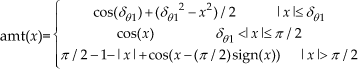
Assume the function amt(x) is (9); then, its derivative is (10):

Let AM(k) denote the attractive moment imposed by the OWRpointi at the current time tk; then, AM(k) is designed as follows.
If the OWRpointi is not T or else if its distance from PRi is larger than DS, then AM(k) is only required to make Ri's PMDline face the OWRpointi. As with when Ri's PMDline is facing the OWRpointi, the objective for Ri in moving closely to the OWRpointi can be fulfilled by the motion vector (Sxi(k+1),Syi(k+1)) T . Thus, AM(k) is designed as (11) in this case:.

If the OWRpointi is T and its distance from PRi is not larger than DS, AM(k) is required to influence both Ri's PMDline and position so that Ri can reach Ti exactly while having as similar a posture to T as is possible. Thus, AM(k) is designed as (12) in this case:

Let (Δ2β Ri (k), Δ2xRi(k), Δ2yRi(k)) T denote the expected vector to increase AM(k); then, it is the gradient of AM(k). When the OWRpointi is not T or its distance from PRi is larger than DS:

When the OWRpointi is Ti and its distance from PRi is not larger than DS:

4.3 Repulsive Moments and Motion Controller
Suppose that G is a dangerous wall representative point of Ri at the current time tk and that PM(k) is the repulsive moment generated by G at tk.
When R has no coordinated companion at present, PM(k) is only required to cause Ri's PMDline to move away from G. As with when Ri's PMDline is away from G, the objective for R in moving away from G can be fulfilled by the motion vector (Sxi(k+1), Syi(k+1)) T . Thus, PM(k) is designed as (15) in this case:

where λ p =(DS-|PRiG|)/DS, which increases with any decrease of |PRiG| for the reason that the lower that | PRiG | is, the larger that the repulsive moment is required to be, so that Ri's PMDline can move away from G quickly.
When R has coordinated companions, PM(k) is required to influence Ri's position but not the PMDline so that the influence of the coordinated moments on Ri's position can be weakened and so that R will not move too closely to G. Accordingly, PM(k) is designed as (16) in this case:

where (xD, yD) T is the coordinates of the end-point of the directed segment with a start-point G, a direction angle β(G, PRi) and a length DS.
Let (Δ3β Ri (k), Δ3x Ri (k), Δ3y Ri (k)) T denote the expected vector to increase PM(k); then, it is the gradient of PM(k). When R i has no coordinated companion:

When Ri has coordinated companions:

(ΣΔ3β Ri (k), ΣΔ3x Ri (k), ΣΔ3y Ri (k)) T denotes the sum of the gradients of all repulsivemoments acting on R i , where when R i has no dangerous wall representative point at t k , (ΣΔ3β Ri (k), ΣΔ3x Ri (k), ΣΔ3y Ri (k)) T =(0, 0, 0) T .
The motion controller of Ri using artificial moments for multi-robot path-planning is designed as (19), (21), (22):
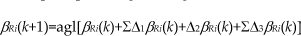
Let:

If

Otherwise:

From (2)–(22), we can conclude that the proposed motion controller can make a robot enter and pass through narrow passages. Although the effects of attractive and repulsive moments may be cancelled out by each other when R is close to a narrow passage, R can still enter the passage through the motion vector (Sxi(k+1), Syi(k+1)) T .
The controller can also make Ri reach a target with obstacles nearby. As with when Ri is close to Ti, (Sxi(k+1), Syi(k+1)) T is zero, which means that repulsive moments cannot influence Ri's motion. As a result, Ri can reach Ti under the influence of the attractive moment generated by Ti.
When Ri has no coordinated companion, the controller will make Ri move under the guidance of its OWRpoints at its full speed for almost of the time. As such, no problem similar to the “local minimum” problem exists in the controller as it is impossible for Ri to stay at a “local minimum” point or in a small region.
5. Algorithm for multi-robot path-planning
Although the proposed motion controller has many advantages, it still has certain problems.
One is that where the OWRpointi is not Ti or else its distance from PRi is larger than DS, the controller may cause Ri to move away from the OWRpointi if Ri has a dangerous wall representative point G satisfying (23), as shown in Figure 3(a):


(a) Ri moves away from the OWRpointi; (b) Ri cannot achieve the same posture as that of Ti as much as possible. (c) The conflict between Ri and Rj cannot be solved effectively.
The reasons for this are that if (23) is satisfied, Ri 's PMDline direction may not be changed by the controller since the sign of agl (β Ri -β(PRi, OWRpointi)) will be opposite to that of agl (β Ri -β(G,PRi)), as shown in Figure 3(a); as such, the effects of the attractive and repulsive moments may cancel each other out. Accordingly, Ri will move away from the OWRpointi if |agl(β Ri -β(PRiOWRpointi|≥π/2. In this situation, the method for avoiding the problem set out above is to let β Ri (k) be agl(β(PRi, OWRpointi)+δθ1) if the OWRpointi is T or else after lettingβ Ri (k)=agl(β(PRi, OWRpointi)+δθ1), Ri 's PMDline has no intersection with the knowledge obstacle wall on which the OWRpointi lies; otherwise, let β Ri (k) be agl(β(PRi, OWRpointi)-δθ1).
A second problem is that in the case where the OWRpointi is Ti and its distance from PRi is not larger than DS, the controller may not cause Ri to achieve the same posture as that of Ti as much as possible, if Ri has a dangerous wall representative point G satisfying (24), as shown in Figure 3(b).

The reasons are similar to that of the first. In this case, the method for avoiding the problem is to let β Ri (k) be β Ti (k).
A third problem is that where the OWRpointi is Ti and the distance between PRi and Ti is not larger than DS, if Rj is a coordinated companion of Ri and |agl(β Ti -β Rj )| <δθ2, as shown in Figure 3(c), then the controller may not resolve the conflicts between Ri and Rj. The reasons for this are that as the direction of Ri 's PMDline may be the same as that of Ti's PMDline under the influence of the attractive moment generated by Ti, it is concluded that there is no marked trend for them to move towards each other. As a result, the coordinated moment generated by Ri will only allow Rj to maintain a certain safe distance from Ri but it will not guide Rj in bypassing Ri. In this situation, the method for avoiding the problem is to let β Ti (k)=agl(β Ti (k)+π).
After the above-mentioned pre-processes, the proposed controller performs well in various situations. The algorithm for the local path-planning of multi-robots is then given as follows:
1: Set the values of the parameters in the control system; initialize the shared environment and the sets of robots, targets and knowledge obstacle walls; let tk =t0.
2: For each robot that has not reached its target, remove or set artificial obstacle segments until no such work can be done.
3: For each robot Ri, if it has not reached Ti or else has coordinated companions, then go to step 4. Otherwise, its position and PMDline will not be changed.
4: Obtain the OWRpointi and all dangerous wall representative points of Ri.
5: In the case where the OWRpointi is T and its distance from PRi is not larger than DS, if Ri has a coordinated companion Rj and |agl(β Ti -β Rj )|<δθ2, then let β Ti =agl(β Ti +π); otherwise, if Ti's PMDline direction is not that at t0, then let β Ti be that at t0.
6: If the OWRpointi is not Ti or else its distance from PRi is larger than DS, then if Ri has a dangerous wall representative pointG satisfying (23), let βRi(k)=agl(β(PRi, OWRpointi)±δθ1). Otherwise, if Ri has a dangerous wall representative point G satisfying (24), let βRi(k)= βTi(k).
7: Move a step to the next position under the control of the proposed motion controller. Update the current time as tk +1.
8: If all of the robots have reached their targets, then stop; otherwise, update their knowledge obstacle walls and let tk = tk +1; then, return to step 2.
6. Simulations and analysis
In order to demonstrate the feasibility of the proposed method, extensive simulations have been carried out and two of them are given in what follows. In the simulations, no robot has a priori knowledge about the environment or other robots. The parameters are: DR=0.4, DV=3.5, DS=1, DM=SR=0.24, λ1=0.5, λ2=0.8, δθ1=π/90 and δθ2=π/3. A simulation will terminate automatically if the distance from the boundary of a robot to that of another one (or an obstacle) is less than 0.05.
The path-planning of two robots in a complicated environment is shown in Figure 4 where (including Figure 5) short segments on obstacles are N-type artificial obstacle segments. From Figure 4, we can see that the two robots encounter each other in a narrow passage whose width is only 2DS =2, but the conflict between them is solved quickly. The simulation verifies that the method is effective in solving the conflicts between robots in narrow passages and that robots will not be trapped in complicated environments.
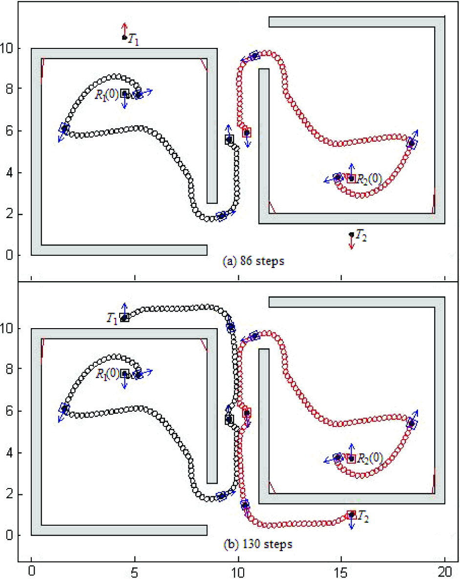
Path-planning of two robots with 130 steps
The path-planning of three robots in a complicated environment is shown in Figure 5, where T3 is in the middle of a narrow passage whose width is also 2DS=2, and R3 is at T3 at the initial time.
Figure 5 (a) and (b) present the situations in solving the conflicts between the robots at the entrance of a narrow passage and in the middle of the passage, respectively. The simulation verifies, again, that the method is effective for the path-planning of multi-robots in complicated environments.

Path-planning of three robots with 149 steps
From Figures 4 and 5, we can see that although the path travelled by each robot may not be the optimal one, it is sure to be a sub-optimal one. As such, the method can optimize the path travelled by each robot.
7. Conclusions
From the discussion and simulations given in this paper, we can arrive at the following conclusions.
The proposed method meets the requirements of the real-time property for the following reasons. Firstly, all of the computations involved in the method are spatially distributed and their complexity is bounded regardless of the number of robots. Secondly, it needs almost no pre-processing of the environment, no consideration of the safe distance of robots and no explicit communication. Thirdly, the computational complexity of OWRpoints is low.
Compared with the traditional APF method, the proposed motion controller has certain advantages as follows. Firstly, under its control, a robot will not be trapped in a complicated environment, can enter and pass through narrow passages, can reach a target with obstacles nearby, and can achieve the same posture as that of its target as much as possible when it reaches its target. Secondly, it can resolve the conflicts between robots while no other techniques - such as priorities and negotiation - are needed and it can minimize other robots' influences on a given robot's motion.
The proposed method can optimize the path travelled by each robot as each robot's motion is under the guidance of its OWRpoints and other robots' influences are minimized by coordinated moments.
A disadvantage is that the proposed method may find it difficult to solve the conflicts between robots in passages narrower than 2DS or in a dynamical environment. In the future, we will try our best to overcome these disadvantages.
Footnotes
8. Acknowledgments
The research reported in this paper was supported by the NSF of China under Grant No. 60874017, the State Key Laboratory of Robotics and System (HIT) under Grant No. SKLRS-2011-MS-03 and the Special Research Foundation of Liaoning University of Science and Technology under Grant No. 2012RC01.