A Study of Force and Position Tracking Control for Robot Contact with an Arbitrarily Inclined Plane

Abstract

This paper proposes an adaptive impedance control method for a robot's end-effector while it slides steadily on an arbitrarily inclined panel; it concentrates on robot force position tracking control for the inclined plane with an unknown normal direction and varying environmental damping and stiffness. The proposed control strategy uses the Recursive Least Squares (RLS) algorithm to estimate environmental damping and stiffness parameters during the impact-contact process between the robot and the environment. It achieves the expected posture adjustment of the robot's end-effector based on the measured contact torques and, during the robot's end-effector's sliding on the inclined plane, a fuzzy control is developed to adjust the robot impedance model parameters on-line and adaptively for changes in environmental damping and stiffness. The designed robot force position control method is robust to the changes of the environmental parameters but the implementation of the proposed control algorithms is simple. Finally, experiments demonstrate the effectiveness of the proposed method.

1. Introduction

Research into force/position control between robots and unknown environments is currently a hot topic. The focus is mainly on improving the robot control system's performance while the environment's geometry parameters and dynamics parameters (damping and stiffness) are unknown or changing; it aims to increase the robustness of the robot force/position control. This paper focuses on robot contact with an arbitrarily inclined plane. The force/position control between robots and inclined planes has been studied by scholars recently. Karayiannidis Y. and Doulgeri Z. proposed the sloping surface normal direction vector online adaptive calculation based on the robot's joints' angle displacement and velocity while its algorithms slowly converge.^[1–3] In other papers, they designed an algorithm that can achieve sloping surface normal direction estimation and force/position control at the same time, based on the robot's joint displacement and the contact force applied at the robot's end-effector. The contact surface tangential velocity is constant but the algorithm is too complex to be achieved in projects.^[4–6] Furthermore, they used the approximation capabilities of neural networks to achieve the force and position trajectory tracking of a robot in compliant contact with a flat surface under non-parametric uncertainties existing in the dynamic and contact model.^[7] Olsson T. et al. combine force sensing, visual perception and displacement sensors to achieve robot force/position control along arbitrary slopes.^[8] Erickson D. et al. compare several methods of parameter (damping and stiffness) estimation for unknown environments and summarize the advantages and disadvantages of each method for the robot's force/position control.^[9] Mallapragada V. et al. try to estimate environmental damping and stiffness with RLS and design a PI controller to compensate for the environmental parameters so as to estimate errors based on neural networks.^[10]

This article introduces an adaptive impedance control for the force and position tracking control between a robot and an arbitrarily inclined plane. First, in order to stimulate environmental dynamic features - commanding the robot's end-effector to collide with the contact surface - it improves the precision of the environmental damping and stiffness estimation by RLS. Second, when the contact is stable, we adjust the posture of robot's end-effector to the expected value according to the contact torque. Finally, during the sliding of the robot's end-effector on the inclined plane, the changes of force and position are tiny compared to the measuring noise. This article introduces a fuzzy control based on position and contact force feedback so as to modify the damping and stiffness parameter of the robot impedance model online, being adaptive to environmental damping and variances of stiffness.

2. Robot impedance control model

Hogan, H. proposed a robot impedance control method in 1985. This method makes the robot end-effector's force/position control equivalent to the Spring-Weight-Damping model. It determines the relationship between the robot's end-effector displacement and the contact force by adjusting inertial, damping and stiffness parameters. Robot impedance control overcomes the disadvantages of frequently switching between the force control and position control of the robot's force position control. The ideal model of robot impedance control is:^[11]

$M_{\mathrm{d}}\left[\stackrel{.}{X}(t)-{\stackrel{.}{X}}_{\mathrm{d}}\right]+B_{\mathrm{d}}\left[\stackrel{.}{X}(t)-{\stackrel{.}{X}}_{\mathrm{d}}\right]+K_{\mathrm{d}}\left[X(t)-X_{\mathrm{d}}\right]=E(t)$

(1)

where X(t) refers to the robot's current position, Xd refers to the robot end-effector's expected position, M _d refers to the robot impedance models ideal inertial, B _d refers to ideal damp, K _d refers to ideal stiffness. B _d, K _d and M _d should be a l*l positive definite diagonal matrix in order to achieve decoupling control. l refers to the dimension of the robot work space, E (t)= F _d− F _e(t), F _d refers to robot end-effector's expected contact force, F _e(t) refers to the actual contact force. Robot impedance control seeks to achieve the robot end-effector's expected position and force control by adjusting M _d, B _d and K _d. The environment in robot impedance control is usually regarded as a spring-damping model: ^[10]

$F_{\mathrm{e}}=B_{\mathrm{e}}\left[\stackrel{.}{X}\text{(}t\text{)}-{\stackrel{.}{X}}_{\mathrm{e}}\right]+K_{\mathrm{e}}\left[X\text{(}t\text{)}-X_{\mathrm{e}}\right]$

(2)

In the formula, B _e and K _e refer to environmental damping and stiffness respectively, X _e refers as the initial position in the environment, X (t) is the position when the environment is changed and F _e represents the total external force applied in the environment.

3. The influence of environmental parameters on robot impedance control

When robot impedance control is used for force/position control between the robot and the environment, the environmental parameters are unknown or changing or else cause the system's dynamic and static performance to decrease. Research into environmental stiffness and the influence of damping on the force/position control between the robot and the environment is the basis of using robot impedance control.^[12–13]

3.1 Stable error influence

When robot's end-effector is in contact with the environment and the system is in steady state then according to robot impedance model Eq(1), we get F_e-F_d=K_d(X-X_d) while and the environment model Eq(2) yields F_e=K_e(X-X_e). In order to satisfy F _d =F _e , let X_d = X_e + F_d/K_e. Define the robot reference trajectory as X =X +FdK, then replacing Xd in Eq (1) by X_r yields M_dẌ(t) + B_dẊ(t) + (K _e + K_d)(X(t)-X_r) = 0. When t→∞, then the robot end-effector's displacement X (t) → X _r = X _e + Fd/Ke and the contact force between the robot and the end-effector and the environment is F ( t ) = K _e(X-X_e)→F_d, then the robot end-effector's expected contact force and position control are achieved at the same time. Meanwhile, in a practical application, environmental stiffness K _e is usually unknown or changing, and so it should be calculated online.

3.2 Dynamic performance influence

Substituting Eq(2) into Eq(1), the interaction between the robot's end-effector and the environment can be equivalent to a second-order system and the damping coefficient ξ and un-damped vibration angular frequency wn should satisfy^[10] ${\mathrm{w}}_{\mathrm{n}}=\sqrt{\frac{{\mathrm{K}}_{\mathrm{d}}+{\mathrm{K}}_{\mathrm{e}}}{{\mathrm{M}}_{\mathrm{d}}}}$ , $\xi =\frac{{\mathrm{B}}_{\mathrm{d}}+{\mathrm{B}}_{\mathrm{e}}}{2\sqrt{({\mathrm{K}}_{\mathrm{d}}+{\mathrm{K}}_{\mathrm{e}}){\mathrm{M}}_{\mathrm{d}}}}$ , where the parameters W_n and ξ determine the dynamic performance of the second-order system. When the variation of the environmental parameters (K_e, B_e) causes the changes of (W_n, ξ), in order to maintain the expected dynamic performance of force/position control between the robot and the environment, the impedance control model parameters (M_d, K_d, B_d) should be adjusted according to variations in the environment. One of the adjustment methods is to measure (K_e, B_e) in real-time or else calculate (K_e,B_e) according to the environment model, modifying (M_d, K_d, B_d) to compensate for the environmental changes. Another adjustment method is to design a smart controller to adjust (M_d,K_d,B_d) online based on the robot's real-time position and contact force feedback; it reduces the influence of changes of the environmental parameters on the system's dynamic performance. The proposed robot force/position control method in this article applies the two adjustment methods to improve the control system's self-adaptive ability in relation to unknown (changing) environmental parameters during different phases of the interaction between the robot and the environment.

4. Robot's force position control along the inclined plane

Robot force position control along the inclined plane mainly contains the force control along the normal direction of the contact surface and the position control in the contact surface's tangential direction. At present, the robot impedance control which is used to achieve robot force position tracking control between the robot and the environment mainly focuses on uncertainties or else changing environmental damping and stiffness.^[14–15] In order to satisfy these demands, this article estimates the initial value of the environmental parameters (B_e, K_e) with RLS during the impact-contact process between the robot and the environments when the contact becomes steadily; it calculates the robot posture rotation matrix according to the contact torque. During the robot's end-effector's sliding on the inclined plane, we design the fuzzy turning mechanism to modify (B_d, K_d) online in order to achieve adaptive robot impedance control for the variance of the environmental parameters (B_e,K_e).

4.1 Estimation of the initial values of the environmental parameters (B_e, K_e)

In the environmental model Eq (2), let δX=X(t)-Xe yield F = BδSẊ + KδX, whereby it is discretized as^[11] $F=\left[B(\frac{2}{T})(\frac{1-z^{-1}}{1+z^{-1}})+K\right]\text{δ}X$ . T refers to the sampling time, such that the corresponding difference equation is:

$\begin{array}{l}F[\mathrm{k}]+F[\mathrm{k}-1]=\left(B(\frac{2}{\mathrm{T}})+K\right)\text{δ}X[\mathrm{k}]+\left(K-B(\frac{2}{\mathrm{T}})\right)\text{δ}X[\mathrm{k}-1]\\ k=1,2,\dots ,\propto ,\end{array}$

which it can be written as: Y[k] = φT [k]θ[k], where

$\begin{array}{l}\theta \left[\mathrm{k}\right]={\left[A_1\left[\mathrm{k}\right] A_2\left[\mathrm{k}\right]\right]}^{\mathrm{T}},A_1=B(\frac{2}{T})+K,A_2=K-B(\frac{2}{\mathrm{T}}),\\ \mathrm{\varphi }\left[\mathrm{k}\right]={\left[\text{δ}X\left[\mathrm{k}\right]\text{ δ}X\left[\mathrm{k}-1\right]\right]}^{\mathrm{T}},Y\left[\mathrm{k}\right]=F\left[\mathrm{k}\right]+F\left[\mathrm{k}-1\right].\end{array}$

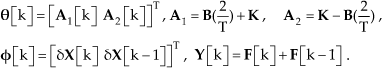
Applying the RLS to calculate θ[k]: θ[k]=θ[k−1]+G[k]-φ^T[k]θ[k−1]) the gain factor, $G[\mathrm{k}]=\frac{P[\mathrm{k}-1]\mathrm{\Phi }[\mathrm{k}]}{\lambda +{\mathrm{\Phi }}^{\mathrm{T}}[\mathrm{k}]P[\mathrm{k}-1]\mathrm{\Phi }[\mathrm{k}]}$ , P[k] refers to the parameters for estimating the covariance matrix and $P[\mathrm{k}]=\frac{1}{\lambda }\left[P[\mathrm{k}-1]-\frac{P[\mathrm{k}-1]\mathrm{\Phi }[\mathrm{k}]{\mathrm{\Phi }}^{\mathrm{T}}[\mathrm{k}]P[\mathrm{k}-1]}{\lambda +{\mathrm{\Phi }}^{\mathrm{T}}[\mathrm{k}]P[\mathrm{k}-1]\mathrm{\Phi }[\mathrm{k}]}\right]$ , λ the forgetting factor and its value is 0.9. In the above iterative computations of θ[k], if the changes of θ[k] are smaller than the user's set threshold value and the value of θ[k] is regarded as stable, then according to A1 and A2, we can get the formula for (Be, Ke): ${\widehat{B}}_{\mathrm{e}}(\mathrm{k})=\mathrm{T}\left(\frac{A_1-A_2}{4}\right),{\widehat{K}}_{\mathrm{e}}(\mathrm{k})=\frac{A_1+A_2}{2}$ . Maintaining the control system in an over-damping state during the impact-contact, we can make the estimation of (Be, Ke) more precise.

4.2 Robot end-effector's velocity control along the inclined plane

The sliding of the robot's end-effector on the inclined plane is shown in figure 1. V_n refers to the velocity of the robot's end-effector. We adjust the robot's posture relative to the inclined plane when it is in contact with it and it is no longer necessary to make adjustments when the robot's end-effector is sliding on the inclined plane. Accordingly, in this article the posture is adjusted according to the contact torque when the contact between the robot's end-effector and the inclined plane is kept stable. The sliding of the robot's end-effector on the inclined plane is shown in figure 1. F n refers to the force in the inclined plane's normal direction and F _f refers to the friction force. When the robot's end-effector begins to make contact with the inclined plane in a steady state, the trend of relative motion is faint and F _f can be omitted. In the current posture, F _n causes the torque M_n(k) at the robot's end-effector. We assume that F _n causes a torque M _d at the robot's end-effector in the expected posture and define e_m(k)=‖M_d-M_n(k)‖; thus, the rotation matrix for the adjustment of the posture of the robot's end-effector in the robot's tool coordinate frame is^TR(k + 1) (the force sensor coordinate frame coincides with the robot's tool coordinate frame) ^[16]:

${ }^{\mathrm{T}}R\mathrm{T}(\mathrm{k}+1)=I+\frac{\sin (\theta )}{\Vert \mathrm{u}\Vert }S(\mathrm{u})+\frac{1-\cos (\theta )}{{\Vert \mathrm{u}\Vert }^2}S{(\mathrm{u})}^2,k=0,1,2,\dots ,N,$

where u and θ refer to the equivalent rotation axis and rotation angles, such that the expression of S(u) is described in [16], and $\theta (\mathrm{k}+1)={\mathrm{k}}_{\text{θ}}\mid {\mathrm{e}}_{\mathrm{m}}(\mathrm{k})\mid$ , $\mathrm{u}(\mathrm{k}+1)=\mathrm{u}(\mathrm{k})+{\mathrm{k}}_{\mathrm{m}}\frac{{\mathrm{e}}_{\mathrm{m}}(\mathrm{k})}{\mid {\mathrm{e}}_{\mathrm{m}}(\mathrm{k})\mid }$ , k_m and k_θ are constant. In the robot's basic coordinate system, ${}^{\mathrm{T}}R(\mathrm{k}+1)$ is rewritten as ${}_{}^{\mathrm{b}}R(\mathrm{k}+1)={}_{\mathrm{T}}^{\mathrm{b}}R(\mathrm{k}){}_{}^{\mathrm{T}}R(\mathrm{k}+1){}_{\mathrm{T}}^{\mathrm{b}}R{(\mathrm{k})}^{-1}$ , where ${}_{\mathrm{T}}^{\mathrm{b}}R$ refers to the robot's end-effector current posture matrix. Substituting ${}_{}^{\mathrm{b}}T(\mathrm{k}+1)$ for the robot's inverse kinematics, we can get the robot's joint angle displacement in the expected posture.

Figure 1.

Robot contact with the inclined plane

The robot's end-effector's translational velocity in the inclined plane can be described as ^wv(k) = ^wv_t(k) + ^wv_n(k), where k is the sampling period k=0,1,2,…, the superscript w represents the robot workplace coordinate frame, ^wv_t(k) is the velocity of the robot's end-effector along the inclined plane, ^wv_t(k) = v_user(k)^wt(k)‖^wt(k)‖⁻¹, v_user(k) is the user's defined absolute velocity, ^wt(i) = ^wP(i + 1)-^wP(i) is the difference between the robot's adjacent position, ^wv_n(k) is the velocity in the inclined plane's normal direction and ^wv(k) = ‖^wv_norm(k)|^wo_d(k) where ^wo_d(k) is the normal unit vector of the inclined plane. the calculation of ^wv_norm(k) is presented below.

We define the robot impedance control model as ${\mathrm{M}}_{\mathrm{d}}(\stackrel{.}{x}-{\stackrel{.}{x}}_{\mathrm{d}})+{\mathrm{B}}_{\mathrm{d}}(\stackrel{.}{x}-{\stackrel{.}{x}}_{\mathrm{d}})={\mathrm{K}}_{\mathrm{f}}(\mathrm{F}-{\mathrm{F}}_{\mathrm{d}})$ , where the parameters are the same as with Eq(1). We get X = -M⁻¹_dB_dX + Bd⁻¹K_f(F-F_d) and solving the above differential equation yields:

$\mathrm{X}(\mathrm{t})={\mathrm{e}}^{-{\mathrm{M}}_{\mathrm{d}}^{\text{-1}}{\mathrm{B}}_{\mathrm{d}}\mathrm{X}(0)}+{\displaystyle {\int }_0^t{\mathrm{e}}^{-{\mathrm{M}}_{\mathrm{d}}^{\text{-1}}{\mathrm{B}}_{\mathrm{d}}(t-\tau )}{\mathrm{B}}_{\mathrm{d}}^{\text{-1}}{\mathrm{K}}_{\mathrm{f}}(\mathrm{F}-{\mathrm{F}}_{\mathrm{d}})\mathrm{d}\tau }$

(3)

where t is time for the discrete process of Eq(3) with the sampling period $\mathrm{\Delta }\mathrm{t}$ at time k, given that ${\mathrm{M}}_{\mathrm{d}}$ , ${\mathrm{B}}_{\mathrm{d}}$ , ${\mathrm{K}}_{\mathrm{f}}$ , F and ${\mathrm{F}}_{\mathrm{d}}$ are constant parameters during the sample period ( $\mathrm{\Delta }\mathrm{t}(\mathrm{k}-1)\le \mathrm{t}<\mathrm{\Delta }\mathrm{t}\mathrm{k}$ ), we define $\mathrm{X}(\mathrm{k})=\mathrm{X}(\mathrm{t}){\mid }_{\mathrm{t}=\mathrm{\Delta }\mathrm{t}\mathrm{k}}$ where the recursive computation of X is $\mathrm{X}(\mathrm{k})={\mathrm{e}}^{-{\mathrm{M}}_{\mathrm{d}}^{\text{-1}}{\mathrm{B}}_{\mathrm{d}}\mathrm{\Delta }\mathrm{t}}\mathrm{X}(\mathrm{k}-1)-\mathrm{\Phi }$ ,where $\mathrm{\Phi }=({\mathrm{e}}^{-{\mathrm{M}}_{\mathrm{d}}^{\text{-1}}{\mathrm{B}}_{\mathrm{d}}\mathrm{\Delta }\mathrm{t}}-\mathrm{I}){\mathrm{B}}_{\mathrm{d}}^{\text{-1}}{\mathrm{K}}_{\mathrm{f}}(\mathrm{F}(\mathrm{k})-{\mathrm{F}}_{\mathrm{d}})$ since $X=\stackrel{.}{x}-{\stackrel{.}{x}}_{\mathrm{d}}$ and ${\stackrel{.}{x}}_{\mathrm{d}}=0$ in the inclined plane's normal direction, adding the force error integration to reduce force error in the system's steady state. We define the robotic end-effector's velocity in the normal direction as

${ }^{\mathrm{w}}\mathrm{v}{}_{\text{norm}}(\mathrm{k})=\stackrel{.}{x}(\mathrm{k})={\mathrm{e}}^{-{\mathrm{M}}_{\mathrm{d}}^{-1}{\mathrm{B}}_{\mathrm{d}}\mathrm{\Delta }\mathrm{t}}\stackrel{.}{x}(\mathrm{k}-1)-\mathrm{\Phi }+{\mathrm{K}}_{\mathrm{i}}{\displaystyle \sum _{\mathrm{n}=1}^{\mathrm{k}}[\mathrm{F}(\mathrm{n})-{\mathrm{F}}_{\mathrm{d}}],}$

where K_i ∈ R^3*3 is the contact force feedback error factor.

4.3 Apply the fuzzy control for the robot impedance control

When adjusting the robot's end-effector to the expected posture, the vector unit N along the contact surface's normal direction can be calculated; as such, the robot's end-effector stress along vector N is F = F_n = F· N , where F refers to total contact force. We define f_n = ‖F_n‖, f_d = ‖F_d‖ and in impedance control model Eq(1) set B_d=b_dI^l*l, K_d=k_dI^l*l; thus, the robot impedance control model in the direction N can be written as e_f = m_dë_x + b_dė_x + k_de_x, where e_x=x-x_d and e_f=f_n-f_d refer to the displacement error and force error in the N direction. During the robot's end-effector's sliding on the inclined plane, the environmental (the inclined plane) damping and stiffness are changing while the equivalent damping and stiffness of the robot's end-effector vary in different postures. As such, the impedance model parameters need to be adjusted in real-time to be adaptive to the environmental changes. Since the velocity is low in robot force control, only the impedance model's damping and stiffness parameters need to be modified.

The designed robot adaptive impedance control is shown in figure 2. DK and IK refer to the robot's forward and inverse kinematics, such that the robotic end-effector's gravity compensation is intended to make the contact force measurement more precise. ^bR refers to the rotation matrix of the robot's tool coordinate frame to the robot's basic coordinate frame. The fuzzy controller (FLC) achieves the adjustment of the impedance model's parameters (b d, k d) and we can estimate (kd,bd) by mainly scoping for the robot's impedance control in the whole robot work space by trials: k_min ≤ k_d ≥ k_max,

Figure 2.

Robot adaptive impedance control

k_d=k₀+λ_k(k_max-k_min) and setting b =b₀+λ_b(b_max-b_min), k_d=k₀+λ_k(k_max-k_min), where λ_b and λ_k are defined as the damping and stiffness adjustment factors respectively, with ranges from (−1 +1) and b₀andk₀ referring to the initial damping and stiffness parameters in section 3.1. We define the deviation between the robot's current position and its expected trajectory as e_x and its differential value as e_x, the difference between the current contact force and the expected value as e_f, the designed FLC with inputs of e_x and e_f and an output λ_k to adjust the stiffness kd and with inputs ė_x and e_f and outputs λ_b to adjust the damping b_d.

In the experiment, the varying ranges of e_x, ė_f and e_f are [−0.1 0.1]mm, [−100 100]mm/s and [−0.2 0.2]N respectively. We define the domains of e_x, ė_f, e_f, λ_b and λ_k as the same {−5,−4,−3,−2,−1,0,1,2,3,4,5}. There are five fuzzy subsets in the input and output universe of discourse, with membership functions obeying the normal distribution. The fuzzy control rule is shown in table 1. In practice, we create a fuzzy rule table off-line with the real-time force position control based on the contact force measured by the force sensor and the joint angular displacement measured by the joint encoders. We then inquire into the control table according to ė_x, e_x and e_f - through fuzzy quantization, we get λ_k and λ_b. We multiply λ_k and λ_b by their proportional divisors to update (bd, kd) and substitute the new (b_d, k_d) to Eq(1) to yield the displacement ΔX_n(k) in the normal direction of the contact surface; ΔX_n(k) is regarded as displacement compensation added in order to yield the robot reference trajectory X_r(k) to achieve the expected contact force and position tracking control, substituting X_r(k) in the inverse kinematics to yield the robot joint space reference trajectory Θr(k). Finally, in the robot joint space the proportional-derivative control is used to achieve position tracking control.

Table 1.

Fuzzy control rule

λbλk		ef
ex ėx	NB	NB	NS	ZE	PS	PB
	NB	NB	NS	ZE	PS	PS
	NS	NS	NS	ZE	ZE	PS
	ZE	NS	ZE	ZE	ZE	PS
	PS	NS	ZE	ZE	PS	PS
	PB	NS	NS	PS	PS	PB

5. Experiment and its conclusion

The designed experiment is based on a 5-DOF industrial robot with a Wuhan company numerical control HNC-210B controller and a HSV-18 servo-drive as the hardware platform for the robot control system. The software platform is based on the DOS system, the position control cycle is 4ms, the precision of the ATI Delta force sensor used is 0.1N and the sampling frequency is 7KHz, with an aluminium, smooth round stick installed at the robot's end as the probe. The experiment is shown in figure 3. A smooth and elastic wood is fixed at the wall at a given sliding angle - the probe is intended to contact and slide on the wooden plane in the expected posture. For a simple, we define the robot's expected posture as perpendicular to the plane where the expected contact force is 2N in the plane's normal direction and the tangential movement along the plane is controlled by the direction keys on the control panel. In the experiment, the designed force control would not trigger until the contact between the probe and the plane occurred, as the initial contact force is smaller than 2N and the probe moves close to the plane until the contact force rises to 2N. During the probe's contact with the plane, RLS is used to estimate the initial value of the environmental parameters (B_e,K_e) after the contact force becomes stable, adjusting the probe posture according to the contact torque measured (the contact torque should be 0 - in theory - in the expected posture) to make the centre of axis of the probe perpendicular to the plane. Finally, pushing the directional keys on the control panel manually in order to control the movements of the probe along the plane, it first moves along the –x direction and then along the +x, -z directions at the same time in the robot's basic coordinate frame with a velocity of 20mm/s.

Figure 3.

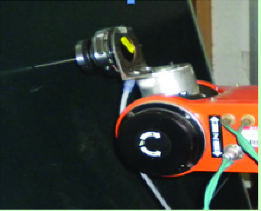
Force/position control along the inclined plane

In the experiment, the force in the normal direction of the plane measured by the sensor is shown in figure 4 (the sampling frequency is 250Hz); after the contact is stable, the deviation between the force in the normal direction and the expected value is within the range of 0.2N (a sudden change in the movement direction may cause the fluctuation of the contact force), the relative displacement of the probe in the robot's base coordinate -x, -y, -z directions is calculated by the robot's joint angular encoders' measure, as shown in figure 5. The displacement changes smoothly in all directions, indicating that the sliding of the probe along the plane is smooth. Since the plane does not coincide completely with the robot's basic coordinate frame, there is some displacement in the -z direction when the probe moves in the –x direction. Since the inclination angle of the fixed plane is arbitrary in the experiment, it can be concluded that the designed control method has achieved the contact force and position tracking control for the robot contact with an arbitrarily inclined plane.

Figure 4.

Contact force in the contact surface's normal direction

Figure 5.

Robot's end-effector's (probe's) displacement in the robot's basic coordinate frame

6. Summary

The design of adaptive impedance control realizes the contact force and position control simultaneously along an arbitrarily inclined plane. it decreases the influence of the unknown inclined plane's normal direction, the uncertainties of environmental damping and stiffness, and the effect of any such changes on the robot's force/position control. The design method has the advantage of: (1) Improving the precision of estimation with RLS, stimulating environmental damping and stiffness estimation with the impact contact; (2) In order to reduce the influence of the contact surface's frictional force on the adjustment of the robot's end-effector posture, we adjust the robot's end-effector to the expected posture according to the contact torque when the robot makes contact stably with the environment. (3) During the robot's end-effector's sliding on the inclined plane, we design the fuzzy controller to modify the damping and stiffness parameters in real-time according to the robot's position error and its deviation and contact force error in order to adapt to the environmental changes and compensate for the impedance model's parameter's estimation error.