Sage Journals: Discover world-class research

Abstract

This paper deals with a problem of road tracking and vehicle positioning based on sequential images captured by a vehicle mounted monocular colour camera. The paper presents a new region-based road tracking method, which is suitable for both structured and unstructured roads. The proposed method is based on our original road segmentation algorithm and estimates road model parameters from measurements obtained by analysis of segmented road region. Although the proposed method is tested over a limited range, evaluation on real image sequences shows promising results for various types of road.

Keywords

Monocular Colour Camera Road Tracking Unstructured Roads Road Segmentation Sequential Monte-Carlo Kalman Filter

1. Introduction

In recent years, together with the increasing capability of capturing devices, vehicle mounted cameras have attracted attention as cheap sensors and vision-based applications using images captured from vehicles are objects of intensive study.

In the field of autonomous vehicles, road geometry recovery and vehicle positioning plays an essential role in path finding and navigational control of the vehicle. One way to accomplish these tasks is to use an image sequence captured by a vehicle mounted camera, and analyse the image sequence by methods of computer vision to extract the necessary information.

The basic idea of to recover road geometry and decide the position of the vehicle from images captured by a monocular camera is to build some kind of road model and fit it to features extracted from the image. There is a group of methods based on stereo-vision [1 –3], but since this paper mainly focuses on methods based on monocular vision, stereo-vision methods are not discussed in detail here. There are also great achievements from the DARPA Grand Challenge [4,5], but the results are achieved by combining camera with LIDAR and other sensors, while here we focus purely on vision-based techniques, mainly because the camera is a completely passive sensor.

Monocular vision-based methods can be further divided into two groups. The first group consists of methods which attempt to detect road boundaries. One type of approach is methods which exploit surface marking to detect road boundaries [6 –8]. Surface marking causes strong edges in gradient image, and edges appears in pairs, which can help to reduce outliers and increase accuracy of road boundary detection. However, such an approach is unusable for unstructured roads (roads without surface marking). The simplest ideas on how to cope with unstructured roads is to use single edges to detect road boundaries [9 –12]. However, edges in gradient image are caused by local changes of intensity and there is no easy way to distinguish between real road boundaries and edges caused by other objects, even if the edge detection is perfect.

An approach opposite to boundary-based methods is the region-based approach. Knowing objects in a form of segmented regions allows us to always decide unique boundaries of the particular object, what is not trivial in the opposite case (find an object from a set of edges), especially in cluttered environments. Region segmentation can also be performed in some cases, when edges cannot be defined and regions differ only in texture. From this point of view, region-based road following should potentially be able to cope not only with structured roads, but also with unstructured roads or rural roads without pavements.

Region-based methods working purely with monocular vision are still very rare compared to boundary-based approach [13,14]. The main reason for this is that the region-based methods are generally more sensitive to lighting conditions, and stable segmentation of the road region is still a very challenging task. Therefore, improvement of road segmentation performance is key to the improvement of region-based road following techniques.

This paper presents a new region-based road tracking method exploiting monocular vision, which is suitable for both structured and unstructured roads. There are two main contributions in this paper. The first one is a sequential Monte-Carlo-based method for extraction of road region from a monocular colour image sequence. The second one is a method for analysis of extracted road region to obtain measurements for estimation of road model parameters. The detailed description of the proposed method is given in the following sections, and experimental evaluation carried out on real image sequences is reported to show performance of the proposed method.

2. Region-Based Road Tracking Method

2.1. Overview of the System

A basic principle behind vision-based road tracking is to define a road model and fit it continuously to some features extracted from the input image. Information about the road which can be obtained by this method strongly depends on the type of the road model. The road is usually modeled by some kind of parametric curve and road tracking in this context can be seen as a problem of how to estimate road model parameters. The most widely used road model approximates left and right road boundaries by quadratic functions [8]. Other methods adopt spline functions [10, 12] or circles [11]. Information which can be obtained using such models is mainly lateral deviation from the road centre, road width, yaw angle with respect to the centre line of road, and road curvature. Furthermore, pitch angle can be obtained on the assumption that the road boundaries are parallel.

In our method, a single quadratic function is adopted, since it is enough to estimate lateral deviation, direction angle and road curvature. As will be seen later, estimation of the road width is also possible, but since road width estimation does not directly depend on the road model in our approach, it is not discussed in detail in this paper.

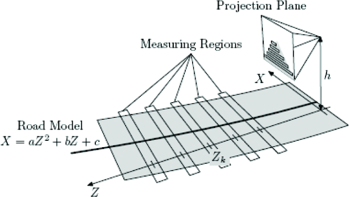
The adopted road model is schematically shown as a top view in Figure 1. The road is modelled as a single quadratic function of the form

X = a Z^{2} + b Z + c

(1)

where a,b,c are parameters to be estimated, and X,Z are coordinates in the coordinate system fixed to the camera and overlaying the road plane.

Lateral deviation ΔX, direction angle μ and road curvature κ can be obtained from the parameters a,b,c by setting Z to origin as follows.

Figure 1.

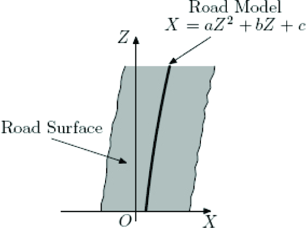
Road Model

Figure 2.

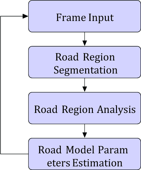
Processing Loop of Road Tracking

Δ X = - c

(2)

µ = - \arctan (b)

(3)

κ = \frac{2 a}{{(b^{2} + 1)}^{\frac{3}{2}}}

(4)

The estimation of the road model parameters a,b,c is schematically shown in Figure 2. Estimation is achieved by continuous repeating of road segmentation, road region analysis and model update steps. Details of the building blocks are described in the following subsections.

2.2. Road Region Segmentation

Road segmentation is a first key step in our method, but generally it is not a trivial task. Since the visual appearance of the road depends on the type of pavement, lighting conditions and many other factors, we need a segmentation algorithm which can adaptively handle changes in the visual appearance of the road.

The key idea in our segmentation method is to estimate the probability density function (PDF) of road pixels from a sequence of observations. We first define five-dimensional feature vector s as

s = {(r, g, b, x, y)}^{T}

(5)

where r,g,b mean colour components and x, y mean pixel position. Our goal is to estimate PDF p(s|u_0:k), where u_0:k stands for sequence of observations. Since roads can take different shapes, and it is very hard to make assumptions about distribution of the colour components p(s|u_0:k) is expected to be strongly non-Gaussian. Therefore, an estimation method which can cope with general distributions is required. In our approach, we adopted a method based on sequential Monte-Carlo estimation [15].

The sequential Monte-Carlo estimation approximates general PDF by using a set of weighted samples, and recursively estimates the sample values and their weights by repeating prediction and update steps. Using the sequential Monte-Carlo estimation, the estimation of road region PDF is performed as follows

Express a PDF of the road region as a set of weighted samples S = {(s_kⁱ,w_kⁱ)}, i = 1…N.

Initialize the sample set S.

For each time step repeat the following:

Draw randomly M samples from sample set S according to importance weights.

Apply transition model of eq.(6) to each drawn sample (See Figure 3(a)).

s_{k}^{(i)} = s_{k - 1}^{(i)} + v

(6)

Here, v denotes a vector of random values with mutually independent normal distributions and zero mean. A simple random-walk type transition model is used, because we have no additional knowledge about transition process.

Set a new weight for each sample according to eq.(7)

w_{k}^{(i)} = p (u_{k}^{(i)} | s_{k}^{(i)})

(7)

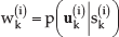
Here, p(u_kⁱ|s_kⁱ) means an observation PDF, which we defined as

p (u_{k}^{(i)} | s_{k}^{(i)}) \propto \exp (- \frac{1}{2} D_{C}^{2})

(8)

D_{C}^{2} = {(c_{k}^{(i)} - u_{k}^{(i)})}^{T} Σ_{m}^{- 1} (c_{k}^{(i)} - u_{k}^{(i)})

(9)

In the equations above, c_k⁽ⁱ⁾ = (r_k⁽ⁱ⁾, g_k⁽ⁱ⁾, b_k⁽ⁱ⁾)^T is a vector of colour components of the sample s_k⁽ⁱ⁾, u_k⁽ⁱ⁾ is a vector of colour components observed in input image at pixel position given by components x_k⁽ⁱ⁾, y_k⁽ⁱ⁾ of the sample s_k⁽ⁱ⁾, and Σ_m is a diagonal matrix of variances of the observation noise. This PDF basically measures distance D_C between colour components of sample and colour components observed in the input image (See Figure 3(b)). High weights are set for the sample when this distance is small, and low weights are set if the distance is large (see Figure 3(c). The size of the circle corresponds to the value of the weight).

Normalize weights such that

Replace set S by the updated weighted samples.

Figure 3.

One Estimation Step of Road Region PDF

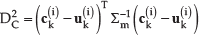
By the above described procedure, road region PDF is estimated in the form of weighted samples. To evaluate p(s|u_0:k)for arbitrary value of s we have adopted some kinds of interpolation. In our method, we used smoothing by Gaussian window, and calculated the value of p(s|u_0:k) for arbitrary s as

p (s | u_{0 : k}) = α \sum_{i = 1}^{N} w_{k}^{(i)} \exp (- \frac{1}{2} {(s - s_{k}^{(i)})}^{T} \sum^{- 1} (s - s_{k}^{(i)}))

(10)

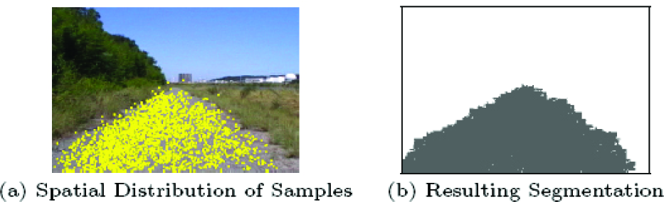
Here Σ is a diagonal matrix of parameters which control the width of the Gaussian window, s_k⁽ⁱ⁾ is a sample from sample set S at discrete time k, w_k⁽ⁱ⁾ is weight assigned to the sample and α is a normalizing coefficient. Segmentation of road region from input image is performed by pixel-wise evaluation of thep(s|u_0:k) and simple thresholding is used to decide road and non-road pixels.

The segmentation algorithm described above can be seen as a kind of tracking method without a priori shape model. The cloud of samples tracks (after initialization) the road region features within the feature space, formed by colour components and spatial coordinates (simple heuristics that a road should be visible at the bottom of the image is used in initialization). By this we obtain a PDF of the road region features in the discrete form, and we use the PDF as a classifier to decide road and non-road pixels.

Figure 4(a) shows an example of spatial distribution of the samples for one frame from a real image sequence. Figure 4(b) shows a segmentation result for this frame, obtained by evaluation of eq.(10). Pixels in output image are set to grey if the value of eq.(10) is above the threshold, and white if the value is below the threshold.

Examples of segmentation results for image sequences with representative frames in Figure 5 are shown in Figure 6. For a more exact evaluation of the segmentation method, we segmented manually all frames for example sequences in Figure 5, and used a Jaccard index to measure the similarity between manually segmented frames and the segmentation results obtained using our method. The Jaccard index for two sets A and B is defined as

J = \frac{| A \cap B |}{| A \cup B |}

(11)

In our case A is a set of road pixels segmented by our segmentation method, and B is a set of road pixels segmented manually. Symbol | | means size of set. Corresponding averages of the Jaccard index for each sequence are summarized in Table 1. As can be seen, the proposed method shows a good performance for different types of road surface, including a road without pavements. A plausible result is obtained also for the sequence with another car in the same traffic line. More detailed description and evaluation results for our segmentation method can be found in our previous report [16].

2.3. Analysis of the Road Region

As is shown in Figure 2, after segmentation of the road region we perform an analysis of the road region to obtain measurements for estimation of the road model parameters. In our method, the analysis of the road region is performed with the help of measuring regions. Basic configuration is shown in Figure 7. Measuring regions are virtual rectangles placed at predefined Z coordinates Z_k, k = 1,…, N and centered at the current road model curve.

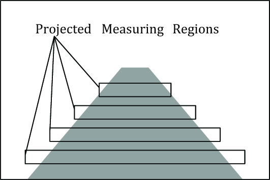
With known camera parameters (perpendicular distance from road surface h, pitch angle, focus length), the measuring regions can be projected to the image plane, and superimposed to the segmented road region. This is schematically shown in Figure 8. Using these projected regions, we calculate measurements for road model parameters' estimation as follows.

Figure 4.

Samples and Resulting Segmentation

Figure 5.

Example of Road Images

Figure 6.

Segmentation Results

Table 1.

Average Jaccard Index $\bar{J}$ for Segmentation of the Sequences in Figure 5(a)-(f)

	(a)	(b)	(c)	(d)	(e)	(f)
J̄	0.82	0.81	0.80	0.91	0.89	0.87

Using the centre point of each measuring region as seed point, we extract all road pixels within the measuring region connected with the seed point by region growing method. If the seed point is a non-road pixel, the measurement is discarded from further processing. Using extracted pixels, we calculate their centre of mass for each measuring region, and use a horizontal coordinate of the centre of mass as a measurement for road model parameters estimation. A vertical coordinate of the measured point is kept fixed at the centre of measuring region. Next we project measured points back into the X,Z coordinate system. By this we obtain a set of N points {X_k,Z_k}with predefined Z_k coordinates, where Nis a number of measuring regions.

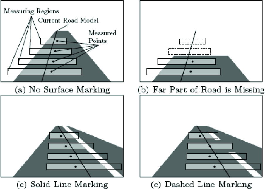
Let us next explain how the extraction of measuring points behaves for different road types. Figure 9 shows schematically typical road situations.

Let us first look in Figure 9(a). The current road model here is closer to the left side of the road, and parts of measuring regions are outside of the road region. Road pixels connected to the centre of the measuring regions are filled with light grey and measured points, calculated as centres of mass of the light grey regions, are shown by black dots. Since the measured points are closer to the road centre, the road model after update would shift to the right, which is a desired behaviour.

Figure 9(b) shows a situation when a far part of road is missing. This can occur when a road is occluded by another car in the traffic line. As was described above, we can decide the measurement to be invalid, if the measuring region is completely outside of the road. This allows us to handle a number of valid measurements and stop the estimation process if the number of valid measured points is insufficient, and no meaningful estimation can be performed.

Another situation is shown in Figure 9(c). Such a situation can occur for roads with multiple traffic lines separated by a solid line. The current road model is shown closer to the right side of the traffic line and a part of the measuring regions is covering a road region of another traffic line. Because the surface marking is not extracted as a road region (see examples in Figure 5), the road pixels of another traffic line are not connected with the centres of the measuring regions. Again, road pixels connected to the centre of each measuring region are shown by light grey and centres of mass of light grey regions are shown by black dots. Measured points appear at positions closer to the centre of traffic line, and the re-estimated model would shift toward the centre of the traffic line as is desired.

Figure 9(d) shows a case of multiple traffic lines separated by dashed line. Because road pixels of each traffic line are not completely separated, only some of the measuring regions behave in the way described for Figure 9(c). The measuring regions which contain completely connected pixels give measured points which are almost in the same position as an original centre of the measuring region. Positions of the measured points for this case are more noisy than in the previous cases, but they still on average tend to be closer to the centre of the current traffic line. Therefore, we will still also be able to estimate plausible road model parameters for this case using an estimation method which can handle such noisy measurements.

As can be understood from this explanation, the road model does not necessarily pass the centre of the road or traffic line. The road model converges to the centre of the road, if the measuring regions are wider than the road-width. If the width of measuring regions is narrower than the road-width, the estimated road model shifts to the position where the measuring regions are completely contained within the road region.

Figure 7.

Measuring Regions

Figure 8.

Projected Measuring Regions

Figure 9.

Points Measured for Different Road Types

2.4. Estimation of Road Model Parameters

By the road region analysis described above, we can obtain a set of measured points for every frame of input image sequence. Such sets of points form a temporal sequence of noisy measurements, and our goal is to estimate parameters a,b,c of the road model eq.(1) from these measurements. An efficient method for how to achieve this, while exploiting the sequential nature of the measurements, is a method based on Kalman filtering [17]. A Kalman filter estimates the internal state of a linear dynamic system from a series of noisy measurements, on the assumption that a system noise and an observation noise have both Gaussian distribution.

In our case, we have implemented a basic Kalman filter described, e.g., in report [18], for a linear system following state and observation equations.

x_{k} = x_{k - 1} + w_{(0, Q)}

(12)

z_{k} = {Hx}_{k - 1} + v_{(0, R)}

(13)

The state vector of the system is formed by the road model parameters x=(a,b,c)^T. The measurements are formed by vector of lateral coordinates of the measured points as z=(X₁,…,X_N)^T where N is a number of measuring regions. According to the road model eq.(1), the observation matrix H can be expressed as

H = (\begin{matrix} Z_{1}^{2} & Z_{1} & 1 \\ ⋮ & ⋮ & ⋮ \\ Z_{N}^{2} & Z_{N} & 1 \end{matrix})

(14)

where Z₁,…,Z_N are fixed longitudinal coordinates of measured points. Since we use fixed Z coordinates, the matrix H is constant, and the relation between parameters (a,b,c)^T and (X₁,‥,X_N)^T is linear.

System noise w_(0,Q) and observation noise v_0,R) both have zero mean, and variance matrices Q and R are set to diagonal matrices with constant elements.

3. Experimental Evaluation and Results

3.1. Test Data

We prepared real image sequences of roads captured from the moving vehicle. The representative frame for each of the test sequences is shown in Figure 10. Since we did not consider exceptional dealing with an insufficient number of measurements in the evaluation, image sequences without another car in the same traffic line were selected.

For each sequence in Figure 10 we prepared a corresponding sequence of ideally segmented road regions. Each frame of these sequences was segmented manually from the original image. Only the own traffic line was segmented for roads with multiple traffic lines. Manually segmented data were used to prepare nominal parameters, as a ground truth for the evaluation experiments.

3.2. Reference Methods

To evaluate the performance of our method, we implemented two reference methods and compared results for each method.

The first reference method is a region-based approach, which performs the same analysis of road region and parameter estimation as the proposed one method, but the segmentation algorithm was replaced by a standard region growing technique. The Euclidean distance of colour components is used as criteria for pixel aggregation, and mean values of colour components are updated every time the new pixel is aggregated. We refer to this method as REF-1 in the following.

The second reference method (REF-2 in the following) uses gradient image to localize single edges, caused by left and right road boundaries, by finding maximal values of gradient norm.

Figure 10.

Test Image Sequences

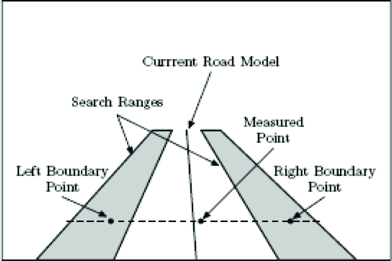
Configuration of the REF-2 is schematically shown in Figure 11. Since we search for positions of local maximum values, we need to limit the search range to reduce outliers. This is achieved by setting search ranges around expected road boundaries. The search ranges are set over left and right side of the expected road, where the positions of ranges are calculated with respect to the current road model. To set search ranges properly we need to make some guess about road width, and the road width was given manually for each test image sequence in our case. After setting the search ranges, horizontal coordinates of left and right boundary points are searched within each search range, where the vertical coordinates are kept fixed in the same positions as described in subsection 2.3. If both left and right boundary points are found, a new candidate point is calculated as a centre point between the boundary points. If no significant peek is found within the left or right search range, the measured point is discarded from the further processing.

3.3. Results

The segmentation algorithm for the proposed method as well as for REF-1 were tuned as follows. The parameters of the segmentation algorithm were first tuned separately for each test sequence to maximize average Jaccard index by eq.(11). Only one parameter, a threshold for the pixel aggregation criteria, have to be tuned for REF-1. Since robustness to parameter tuning is required, and using different parameters for each particular sequence is not desirable, we need to find some common compromise values. In our case, we used averages of the tuned parameters as a compromise values.

The Q_k and R_k of the Kalman filter were first tuned by visual evaluation and fixed to constant values. The same values were used for all methods and all image sequences.

Ground truth (nominal parameters) were created using manually segmented data. The centre points of each ideally segmented region were used as measured points and nominal parameters a_n,b_n,c_n were estimated by the above tuned Kalman filter.

Next, the proposed method, as well as both reference methods, were applied to all test sequences in Figure 10, and sequences of road model parameters a,b,c were estimated. Measuring regions of the same width (slightly wider then the widest road) were used for all sequences in the case of our method a nd REF-1. For REF-2, the road width was given manually, tailored for each test sequence. Figure 12 shows the estimated model back projected to input image for sequence No.2. Both region-based methods give good results, though the REF-1 contains more outliers then the proposed one. On the other hand, it is very difficult to detect plausible features for the edge-based approach in such images, therefore REF-2 gives a very poor result. Examples of reference parameters and parameters estimated for the same sequence are shown in Figure 13.

To compare a,b,c parameters estimated by each method, we defined differences from nominal parameters a_n,b_n,c_n as

Δ a = a - a_{n}; Δ b = b - b_{n}; Δ c = c - c_{n}

(15)

and evaluated these values frame-by-frame for all test sequences. The results are shown as graphs in Figure 14. Maximal values of differences (in sense of absolute values) are summarized into Table 2.

Figure 11.

Candidate Points Detection for REF-2

Figure 12.

Measured Points and Estimated Road Model for frame 400 of Sequence No.2

3.4. Discussion

Let us first look at the results for the proposed method and REF-1. Both methods give very similar results for sequence No.2, but REF-1 gives worse result then REF-2 for No.6. The results for other sequences also show differences in the behaviour of the proposed method and REF-1. Also, Table 2 shows that the proposed method gives smaller Δ than REF-1 in most cases. Such differences are caused by the performance of the segmentation algorithm. As was mentioned in section 3.3, we used same segmentation parameters for all sequences. Consistently with our previous results [16], the proposed segmentation method works well with one set of parameters for various types of roads. Opposite to this, the region growing segmentation used in REF-1 is very sensitive to a proper threshold of the pixel aggregation criteria, and we could not find a common compromise value, giving us good segmentation results for all sequences. This is not surprising if we realise that the region growing with the Euclidean distance as aggregation criteria assumes that colour distribution of the region is an isotropic Gaussian, but our segmentation method can also cope with non-Gaussian distributions. The result of segmentation for the region growing technique can be improved by exploiting a priori knowledge about a scene [19], but since it limits applicability of the method to a particular type of the road scene, the segmentation method which does not rely on such limitations is desirable.

Figure 13.

Example of Nominal Parameters and Estimated Parameters for Sequence No.2

Figure 14.

Differences for Road Model Parameters of Each Test Sequence

Let us next compare the proposed method with the edge-based approach REF-2. As can be seen from the graph in Figure 14, there is almost no significant difference between our method and REF-2 for the road with surface markings on sequence No.6. For sequence No.5, REF-2 gives a significantly different result after frame 350. In this sequence, a guardrail on the left side appears after passing a curve, and a part of the measured points is miss-detected, since the guardrail edge is mistaken with an edge of surface marking.

For the other sequences, most of the data on Table 2 shows that the Δ for the proposed method is smaller than the Δ for REF-2. For the sequence No.3, the graph in Figure 14. shows a big difference of the Δa for REF-2. In this sequence, there is a shadow on the grass in the left side, caused by a bush growing on the higher part of the left slope. Although this shadow does not overlap with the road, REF-2 confuses the strong edges of the shadow with the road boundary, causing a big error of estimated road parameters. An overall look at Table 2 shows that the Δ for the REF-2 sometimes exceeds more than twice the Δ for the proposed method.

Furthermore, the values of road width were explicitly provided for REF-2, and the width of the search ranges shown in Figure 11. was tuned before the experiments. Opposite to this, the measuring regions of the same width were used for all test sequences, and no additional knowledge was provided for our method and REF-1.

Table 2.

Maximal Differences for Each Method

ID	\|Δa\| _max	\|Δb\| _max	\|Δc\| _max
	1.94×10⁻³	6.17×10⁻²	0.50
2	0.79×10⁻³	3.14×10⁻²	0.17
3	1.93×10⁻³	4.23×10⁻²	0.28
4	1.20×10⁻³	5.24×10⁻²	0.27
5	1.12×10⁻³	5.07×10⁻²	0.66
6	0.43×10⁻³	2.53×10⁻²	0.21
(a)Proposed
ID	\|Δa\|_max	\|Δb\|_max	\|Δc\|_max
1	2.09×10⁻³	7.30×10⁻²	0.43
2	0.60×10⁻³	1.70×10⁻²	0.26
3	1.92×10⁻³	4.60×10⁻²	0.51
4	1.21×10⁻³	6.08×10⁻²	0.83
5	1.48×10⁻³	6.92×10⁻²	0.87
6	0.82×10⁻³	4.02×10⁻²	0.56
(b)REF-1
ID	\|Δa\|_max	\|Δb\|_max	\|Δc\|_max
1	1.66×10⁻³	15.4×10⁻²	1.00
2	2.62×10⁻³	7.08×10⁻²	1.15
3	5.28×10⁻³	3.87×10⁻²	0.29
4	3.14×10⁻³	9.94×10⁻²	0.81
5	2.35×10⁻³	8.49×10⁻²	0.75
6	0.44×10⁻³	2.24×10⁻²	0.20
(c) REF-2

Despite this disadvantage, the edge-based approach does not outperform the region-based one.

4. Conclusion and Future Work

This paper dealt with a problem of vision-based road tracking and vehicle positioning. The paper presented a new method for road tracking based on monocular colour images. The proposed method exploits our original road region segmentation algorithm, and measurements for road model estimation are obtained by analysis of the segmented road region. The proposed method does not generally require road surface markings (although the presence of road markings can improve estimation accuracy), therefore it can be used for both structured and unstructured roads. Although the proposed method was evaluated in a limited range, it shows promising results for various types of road.

There are several issues left for future work. Although the road segmentation algorithm can adaptively handle changes of colour appearance of the road, it is still not fully capable of handling shadows. However, there have been promising reports on shadow removal [20] in recent years, and knowledge from such fields can extend the capability of the road segmentation method.

The evaluation presented in this paper required manually segmented road sequences as a ground truth. Preparing such data is a very time consuming task and a more efficient evaluation method is indispensable for evaluation of large databases.

References

Luong

Q.T.

Weber

Koller

Malik

An integrated stereo-based approach to automatic vehicle guidance. In Fifth International Conference on Computer Vision (ICCV'95), pages 52–57, 1995.

Okutomi

Nakano

Maruyama

Hara

Robust estimation of planar regions for visual navigation using sequential stereo images. In EEE International Conference on Robotics and Automation (ICRA'02), volume 4, pages 3321–3327, 2002.

Wedel

Rabe

Badino

Loose

Franke

Cremers

B-spline modeling of road surfaces with an application to free space estimation. Transactions on Intelligent Transportation Systems, 10(4):572–583, 2009.

Thrun

Montemerlo

Dahlkamp

Stavens

Aron

Diebel

Fong

Gale

Halpenny

Hoffmann

Lau

Oakley

C M

Palatucci

Pratt

Stang

Strohband

Dupont

Jendrossek

L E

Koelen

Markey

Rummel

Niekerk

Jensen

Alessandrini

Bradski

G R

Davies

Ettinger

Kaehler

Nefian

A V

Mahoney

Stanley: The robot that won the darpa grand challenge. J. Field Robotics, 23(9):661–692, 2006.

Nefian

A V

Bradski

G R

. Detection of drivable corridors for off-road autonomous navigation. In ICIP, pages 3025–3028, 2006.

Broggi

Robust real-time lane and road detection in critical shadow conditions. In In Proceedings IEEE International Symposium on Computer Vision, Coral Gables, pages 353–358. IEEE Computer Society, 1995.

Lai

A.H.S.

Yung

N.H.C.

Lane detection by orientation and length discrimination. IEEE Transactions on Systems, Man, and Cybernetics, Part B, 30(4):539–548, 2000.

Takahashi

Ninomiya

A method for robust lane marking candidate selection of lane recognition. Systems and Computers in Japan, 31(3):11–19, Mar. 2000.

Wang

Shen

Teoh

E.K.

Lane detection using catmull-rom spline. IEEE International Conference on Intelligent Vehicles, pages 51–57, 1998.

10.

Teoh

E.K.

Wang

Shen

Lane detection using spline model. Pattern Recognition Letters, 21(9):677–689, 2000.

11.

Lakshmanan

Hero

A.O.

Pavement boundary detection via circular shape models. In Proceedings of the IEEE Intelligent Vehicles Symposium 2000, pages 644–649, 2000.

12.

H.R.

Wang

X.D.

Huang

H.W.

K.S.

Fang

A fast and stable lane detection method based on B-spline curve, pages 1036–1040. Ieee, 2009.

13.

Beucher

Bildoeau

Road segmentation and obstacle detection by fast watershed transformation. In Intelligent Vehicles Symposium'94, Paris, France, pages 296–301, Oct. 1994.

14.

Crisman

Thorpe

Scarf: A color vision system that tracks roads and intersections. IEEE Trans. On Robotics and Automation, 9(1):49–58, February 1993.

15.

Doucet

Godsill

S.J.

Andrieu

On sequential monte carlo sampling methods for bayesian filtering. Statistics and Computing, 10(3):197–208, 2000.

16.

Prochazka

Road region segmentation based on sequential monte-carlo estimation. In Proceedings of ICARCV 2008, pages 1305–1310. IEEE, Dec. 2008.

17.

Kalman

R.E.

A new approach to linear filtering and prediction problems. Transactions of the ASME–Journal of Basic Engineering, 82(Series D):35–45, 1960.

18.

Welch

Bishop

An Introduction to the Kalman Filter. Technical Report TR 95-041, University of North Carolina at Chapel Hill, Department of Computer Science, 2006.

19.

Chern

M Y

Cheng

S C

. Finding road boundaries from the unstructured rural road scene. In 16th IPPR Conference on Computer Vision, Graphics and Image Processing (CVGIP 2003), pages 786–793, Aug. 2003.

20.

Finlayson

G.D.

Drew

M.S.

Cheng

Entropy minimization for shadow removal. International Journal of Computer Vision, 85(1):35–57, Oct. 2009.

Road Tracking Method Suitable for Both Unstructured and Structured Roads

Abstract

Keywords

1. Introduction

2. Region-Based Road Tracking Method

2.1. Overview of the System

2.2. Road Region Segmentation

2.3. Analysis of the Road Region

2.4. Estimation of Road Model Parameters

3. Experimental Evaluation and Results

3.1. Test Data

3.2. Reference Methods

3.3. Results

3.4. Discussion

4. Conclusion and Future Work

References