Mobile Robot Collision Avoidance in Human Environments

Abstract

Collision avoidance is a fundamental requirement for mobile robots. Avoiding moving obstacles (also termed dynamic obstacles) with unpredictable direction changes, such as humans, is more challenging than avoiding moving obstacles whose motion can be predicted. Precise information on the future moving directions of humans is unobtainable for use in navigation algorithms. Furthermore, humans should be able to pursue their activities unhindered and without worrying about the robots around them. In this paper, both active and critical regions are used to deal with the uncertainty of human motion. A procedure is introduced to calculate the region sizes based on worst-case avoidance conditions. Next, a novel virtual force field-based mobile robot navigation algorithm (termed QVFF) is presented. This algorithm may be used with both holonomic and nonholonomic robots. It incorporates improved virtual force functions for avoiding moving obstacles and its stability is proven using a piecewise continuous Lyapunov function. Simulation and experimental results are provided for a human walking towards the robot and blocking the path to a goal location. Next, the proposed algorithm is compared with five state-of-the-art navigation algorithms for an environment with one human walking with an unpredictable change in direction. Finally, avoidance results are presented for an environment containing three walking humans. The QVFF algorithm consistently generated collision-free paths to the goal.

1. Introduction

1.1 Challenges of avoiding humans

Avoiding collisions with humans and obstacles is a fundamental requirement for mobile robots, particularly those operating in human environments. The objective of navigation is to plan and control the motion of the robot from its initial position to its goal position, while avoiding obstacles. The navigation problem for mobile robots has been the focus of tremendous research effort. Most of the algorithms for mobile robot navigation are only suitable for avoiding stationary obstacles and/or moving obstacles whose future position and moving direction are predictable, such as other mobile robots. However, avoiding humans is different from avoiding other kinds of obstacles and poses the following additional challenges:

1. Human motion is unpredictable, changing its speed or direction arbitrarily. For example, human motion is holonomic; a human can stop and move sideways without turning, or directly move sideways without stopping. Predicted human positions and moving directions based upon previous human motions are not reliable. Therefore, precise predictions are unavailable, making the navigation problem more difficult.

2. For safety, humans must always possess a higher priority in a navigation system than robots or inanimate objects. Humans should be able to pursue their activities unhindered and without having to watch out for the robots working around them.

3. Considering human emotional reactions, when a robot avoids a human it should not come too close to the human or block the human's path. This can be considered rude behaviour and could also frighten the human, which may cause a sudden action (such as jumping away) leading to human injury.

1.2 Related research

Currently, the majority of navigation algorithms for mobile robots can be classified into two categories. The algorithms in the first category directly provide the collision free path of a robot by assuming the shapes of obstacles are known and their motion is predictable. Furthermore, they typically neglect the robot dynamics. The algorithms in the second category indirectly generate collision free paths by using the current kinematic and geometric information of the robot and any obstacles, such as the distances between obstacles and the robot and the current velocities of obstacles. These algorithms consider the robot dynamics. The recent relevant literature on mobile robot navigation algorithms will now be reviewed.

Algorithms in the first category have the advantage that optimal collision free paths can be found with stationary obstacles or with moving obstacles whose motions are predictable. We will only review the algorithms for avoiding moving obstacles [1–7], since that is the focus of this paper. A “dynamic window” algorithm was proposed in [1]. It employs a window around the robot based on the velocities the robot can reach without causing a collision in the next time interval. Other algorithms [2, 5] assume the obstacles will move with zero acceleration and use their current positions and velocities to build forbidden regions for the robot's velocity. Collision avoidance is accomplished by keeping the robot velocity outside of these regions. Randomized path planning algorithms have also been proposed for avoiding moving obstacles [3, 4]. They exploit randomization to explore large state spaces efficiently. Incremental search planning algorithms are another alternative. The D* algorithm [6] performs a grid-based search incrementally, based on the current positions of the robot and obstacles. Similarly, a predicted collision-free region was combined with the A* algorithm in [7]. These algorithms typically do not work well for obstacles like humans, due to a lack of accurate position/moving direction predictions.

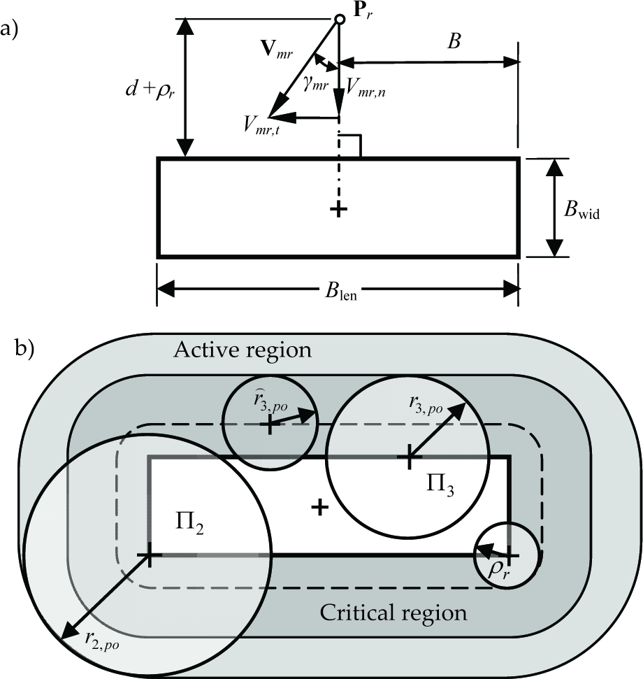
The navigation algorithms in the second category are based on the artificial potential field (APF) (introduced in [10]) or the virtual force field (VFF) (introduced in [11]). These algorithms are normally simple to implement and consume less computational loads than those in the first category. Since virtual forces can be obtained by using the gradient descent method on APFs, they are closely related and belong in the same category. These algorithms assume the existence of a repulsive artificial potential field or a repulsive virtual force surrounding each obstacle to push robots away from the obstacle. An attractive artificial potential field or virtual force is also assumed to be acting to pull the robot to the goal. These algorithms do not directly provide a collision-free path for a robot. The desired accelerations of the robot are given through the dynamic interactions of the robot with the virtual forces. The collision-free path can be obtained by integrating the accelerations with Euler's method. VFF or APF based algorithms have been extensively studied [8–19]. With these algorithms, the force functions or the potential fields are related to the distance from the robot to the goal and the distance to the obstacles. Sometimes they incorporate the velocities of the obstacles and robots in the force functions or potential fields to help the robots avoid dynamic obstacles [8, 10–16, 18–19]. An “active region” surrounding each obstacle is often used to define where the repulsive potential field (or repulsive virtual force) from the obstacle is active. If the robot is inside an obstacle's active region, the repulsive potential field/virtual force is applied to repel the robot away from the obstacle. The attractive potential field may also be active and move the robot towards the goal during navigation. If the robot is outside the region, only the attractive potential field is applied to the robot to pull it towards the goal. The APF/VFF is divided into two parts by the boundary of the active region. In [11, 14] a component tangential to the repulsive component of their potential field is added. This tangential component helps the robot to detour around the obstacle. Similarly, a virtual force that acts perpendicularly to the repulsive force was added in [13]. This force helps the robot to detour around the obstacle and reduces the time required for the robot to reach the goal. In this paper we name this force the detour force. In [13] another region that is very close to the obstacle is utilized. We will refer to this as the critical region. In the critical region a robot may not have sufficient space for complete avoidance, so an alternative to VFF is needed inside this region. It is important to note that methods for systematically designing the size and shape of the active and critical regions are missing from the prior literature.

The APF-based and VFF-based navigation algorithms in the second category are suitable for avoiding moving obstacles whose moving directions are unpredictable, such as humans. This is because the active region provides the space needed to handle the unpredictability. With VFF-based algorithms, if the virtual forces at the boundary of the active region of an obstacle are discontinuous, as in, for example [9, 17], oscillations that waste time and energy may occur as explained in [20]. To both prevent the oscillations and make the motion more efficient, the VFF must be continuous at the edge of the active region.

Another problem with existing APF and VFF-based algorithms, that we will term the collinear condition, was described in [13]. In this condition, an obstacle is located between the robot and the goal and the centres of the robot, obstacle and goal are collinear. The velocity directions of the robot and the obstacle are also on this line (see Figure 1). With conventional VFF algorithms, the attractive force and the repulsive force will all be along this line. Hence, the robot either collides with the obstacle, or is pushed away such that it will never reach its goal. Obviously, the solution is to move the robot sideways. Furthermore, severe path oscillations occur with the existing VFF algorithms whenever the robot, obstacle and goal locations are near to the collinear condition. A non-zero detour force can provide collision avoidance without path oscillations, as shown in Figure 1. This force was not provided in the algorithm in [13]. In [11, 14] a non-zero detour force is provided, however its direction may result in a collision when avoiding a moving human.

Figure 1.

Collinear condition for collision avoidance.

Lastly, proven stability is an unsolved problem for APF-based and VFF-based methods for environments with a variable number of dynamic obstacles. Some researchers have investigated the use of Lyapunov's second method to prove stability. In [11] a pre-known environment with only stationary obstacles was divided into a grid. Using an electrical analogy, each cell of the grid was considered as a resistor, cells occupied by an obstacle were considered as high electric potential, and the goal as ground. Then they established a Lyapunov function, such that the value of the function is the voltage of the cell presently occupied by the robot. The robot is moved to the surrounding cell that has the lowest potential until it reaches the goal. This function is extended for moving obstacles in [14]. However, the number of moving obstacles must be known a priori, otherwise their Lyapunov function will be discontinuous and therefore invalid. The APF algorithm in [16] utilized the modified dipolar potential field for multi-robot navigation. By using this field as the Lyapunov function of the navigation system, a backstepping controller is designed to be globally asymptotically stable. The effectiveness of this method is verified through simulations. However, this method requires perfect knowledge of the environment in order to build the APF and therefore cannot be applied to environments with variable numbers of obstacles. In [17] an APF is designed to be proportional to the distance between the robot and its goal and inversely proportional to the distance between the robot and an obstacle. By using their APF function as a Lyapunov function, they verified the asymptotic stability for avoiding stationary obstacles with one important exception. According to their analysis, under the collinear condition the robot fails to reach the goal.

1.3 Contributions and paper organization

Although significant progress has been made with robot navigation algorithms, several problems have not been addressed in the prior literature, as discussed above. The main contributions of this paper are:

1. A novel VFF-based robot navigation algorithm with improved force functions. It may be used with holonomic and nonholonomic robots to avoid moving obstacles with unpredictable direction changes, including humans.

2. Methods to calculate the sizes of active and critical regions for different obstacles. These methods consider the worst-case avoidance conditions and utilize the shapes, velocity limits and acceleration limits of the obstacle and robot.

3. Proof that the proposed algorithm is stable for variable numbers of stationary and dynamic obstacles.

4. A comparison of the proposed algorithm with five state-of-the-art collision avoidance algorithms for moving obstacles.

It is important to note that our algorithm assumes that the human(s) wish to be independent of the robot(s), unlike in [21] where the focus is on navigation for human-robot social interaction. The organization of the paper is as follows. In Section 2, the methods for establishing the sizes of the active and critical regions are explained. The virtual force functions are designed in Section 3. The stability analysis is presented in Section 4. In Section 5, simulation and experimental results are presented and discussed. Finally, conclusions are drawn in Section 6.

2. Sizing the active and critical regions

2.1 Active and critical regions for a human

The sizes of the two regions will be determined from the robot and human shapes, and velocity and acceleration limits. The active region, termed ${ℂ}_2$ , is defined as the region near the human. If any mobile robot is in ${ℂ}_2$ , the repulsive and detour virtual forces should be activated to make the robot avoid and detour around the human. Therefore, the size of ${ℂ}_2$ is a key issue in the design of a navigation system. It determines how much space is available for the robot to avoid the human. If ${ℂ}_2$ is large, the space available for navigation is wide and the distance between the human and robot will increase, but the time to reach the goal will also increase. The critical region, termed ${ℂ}_3$ , is the region in close proximity to the human and it is very dangerous if a robot intrudes into this region. Within this region, the robot cannot complete the avoidance and should stop to prevent, or at least mitigate, the collision. Any other action made by the robot could worsen the situation. Therefore, when the robot just enters ${ℂ}_3$ , it should be fully decelerated until it is stopped. We define ${ℂ}_1$ as the region that excludes ${ℂ}_2$ and ${ℂ}_3$ for all obstacle(s). ${ℂ}_1$ contains the goal. If the robot is in this region, collision avoidance is unnecessary and the robot simply moves towards its goal.

Since a human's motion is arbitrary, it can change its moving velocity and direction at any time, subject to a limit in linear velocity magnitude. For safety, we need to consider the arbitrary motion made by the human, so the active and critical regions for humans are represented by disk-shaped regions to consider all directions (i.e., assuming the angular velocity of the human is infinite). In the following analysis, we will focus on the design of ${ℂ}_2$ and ${ℂ}_3$ for the human, with consideration of the human's linear velocity limit.

2.2 Size of the critical region for a human

Since a typical mobile robot moves on the floor, the human will be modelled as the projected shape of its body on the floor. The projected shape is highly related to the pose of the human. By modelling a human body as an enclosing cylinder, we can neglect the different poses and simplify the navigation system, while still maintaining safety. The human cylinder shape projected onto the horizontal plane of motion is a disk, as shown in Figure 2. The average step length of a human is 0.8 m [22]. One half of this value will be used as the radius of the human model, i.e. ρ_h= 0.4m.

To simplify the design of the critical region, the shape of the robot will be reduced to a point and the region will be appropriately enlarged. We will use 2D Minkowski addition to sum the disk-shaped human model and the shape of the robot. The projection of the robot onto the floor is modelled as a disk with a radius of ρ _r . The resultant Minkowski sum area (shown enclosed by the dashed-line in Figure 2) is a disk with a radius of ρ+ρ_h. Therefore when the centre of the robot lies on the dashed-circle, the robot will just contact the human model. The shape of the robot can then be regarded as a point in the remaining analysis.

Figure 2.

Design of the critical region for a human.

The size of the critical region is related to the stopping distance, r₃, which ensures that, in the worst-case, robot-human impact will not occur before the robot is stopped, i.e., when the human and robot approach in the collinear condition (defined in Section 1.2) with their maximum velocities V̄ _h and V̄ _mr , as shown in Figure 2. When the robot enters C₃ of the human, it should decelerate with its maximum deceleration magnitude until it stops. The stopping distances are given by:

${\stackrel{⌢}{r}}_3={\bar{\delta }}_{h1}+{\bar{\delta }}_{r1}$

(1)

${\bar{\delta }}_{h1}={\bar{V}}_h\cdot (\mathrm{\Delta }{t}_1+T_s)$

(2)

${\bar{\delta }}_{r1}={\bar{V}}_r{T}_s+\frac{1}{2}{\bar{a}}_{mr}\mathrm{\Delta }{t}_1^2 \text{and}$

(3)

$\mathrm{\Delta }{t}_1={\bar{V}}_{mr}∕{\bar{a}}_{mr}$

(4)

where ${\bar{\delta }}_{r1}$ is the maximum distance required to stop the robot, ${\bar{\delta }}_{h1}$ is the maximum distance that the human could travel towards the robot during the interval Δt₁ + T_s, ā _mrd is the maximum magnitude of the robot deceleration, At is the time required for stopping the robot and T is the sampling period of the navigation system. T_s must be considered due to the lack of position information of the human and robot between sampling instants. r̂₃ also defines a disk, as shown in Figure 2. Mnkowski addition is used to add this disk to the sum of the human and robot disks. Equivalently, the human model can be summed with disk Π₃, as shown. The radius of Π₃ must satisfy:

$r_3>{\stackrel{⌢}{r}}_3+{\rho }_r$

(5)

The combined area defines the critical region for the human. In other words, ${ℂ}_3$ incorporates the stopping distance, the shape of the human and the shape of the robot.

2.3 Size of the active region for a human

The active region of a human should provide the robot(s) with enough room to avoid the human. As previously mentioned, the worst-case is the collinear condition, with the human and robot approaching at their maximum speeds, as shown in greater detail in Figure 3. The initial conditions are as follows: the position and velocity of the robot centre are P_r0 = [P_rx0 P_ry0]^T and V_mr = [V̄ _mr 0]^T, respectively and the position and velocity of the human centre are P_h0=[P_hx0 P_hy0]^T and V _h =[−V̄ _h 0]^T, respectively. The human's velocity here is assumed to be constant. Due to the detour force the robot's velocity will change direction and the robot will move to the point P_r1. The displacement of the robot in the Y-direction must be larger than the radius of ${ℂ}_3$ (i.e. $r_3+{\rho }_h$ ); otherwise the robot will enter ${ℂ}_3$ .

Figure 3.

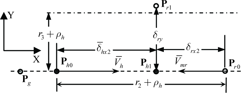
Kinematics of the collinear condition.

Therefore, from Figure 3 the radius of ${ℂ}_2$ (i.e) $r_2+{\rho }_h$ must be larger than the summation of the distances moved by the human and robot in the X-direction before the robot reaches P_r1. If only motion in the X-direction is considered, the radius of Π₂ must satisfy:

$r_2+{\rho }_h>{\bar{\delta }}_{hx2}+{\delta }_{rx2}$

(6)

${\bar{\delta }}_{hx2}=P_{hx}-P_{hx0}={\bar{V}}_h\cdot (\mathrm{\Delta }{t}_2+T_s) \text{and}$

(7)

${\delta }_{rx2}=P_{rx}-P_{rx0}={\bar{V}}_{mr}\cdot (\mathrm{\Delta }{t}_2+T_s)+{\displaystyle {\iint }_{\mathrm{\Delta }{t}_2+T_s}{a}_{mrx}{d}^{2}t}$

(8)

wherea_mrx is the acceleration component of the robot in the X-direction, ${\bar{\delta }}_{hx2}$ and δ _rx2 are as defined in Figure 3 and Δt₂ is the time required for the robot to move by r₃ in the Y direction. However, to avoid a collision the robot must both decelerate in the X-direction (i.e., a_m <0) and accelerate in the Y-direction to reach the dashed-dot line shown in Figure 3. Noting that the velocity of the robot is also limited, we have:

${\delta }_{ry2}={\bar{V}}_{mr}\cdot (\mathrm{\Delta }{t}_2-t_a)+{\displaystyle {\iint }_{t_a}{a}_{mry}dt}>r_3+{\rho }_h$

(9)

where a_mry is the acceleration of the robot in the Y-direction and t_a is the time spent by the robot accelerating from zero velocity to V̄ _mr in the Y-direction. It is impossible to obtain the acceleration in the Y-direction analytically, since it will be different for different algorithms, so Δt₂ cannot be obtained directly. We will estimate Δt₂ by first assuming the robot is driven with maximum acceleration magnitude1, a_mry = ā_mr in the Y-direction. Therefore, (9) is rewritten as:

${\bar{V}}_{mr}\cdot (\mathrm{\Delta }{t}_2-t_a)+\frac{1}{2}{\bar{a}}_{mr}{t}_a{}^2={\delta }_{ry2}>r_3+{\rho }_h$

(10)

So Δt₂ can be estimated with:

$\mathrm{\Delta }{t}_2>\frac{r_3+{\rho }_h-\frac{1}{2}{\bar{a}}_{mr}{t}_a^2}{{\bar{V}}_{mr}}+t_a \text{and}$

(11)

$t_a=\frac{{\bar{V}}_{mr}}{{\bar{a}}_{mr}}$

(12)

where t_a is the acceleration time. The robot acceleration magnitude in the Y-direction will actually be less than ā _mr , since the robot must also decelerate in the X-direction, so the actual Δt₂ will be longer than the computed values and (6) will underestimate the value of r₂. To compensate for this error, we can assume the worst case of a_mrx ≈ 0 and then the conservative estimate for r₂ is given by (7) and:

$r_2>{\bar{\delta }}_{hx2}+{\bar{\delta }}_{rx2}-{\rho }_h \text{and}$

(13)

${\bar{\delta }}_{rx2}={\bar{V}}_{mr}\cdot \left(\mathrm{\Delta }{t}_2+T_s\right).$

(14)

In the analysis presented above, it was assumed that the robot could be directly accelerated sideways (Y-direction). This is true if the robot is holonomic. A nonholonomic robot must be turned π/2 first and then it can be accelerated in the Y-direction. Therefore, the turning time t_turn also needs to be considered. By assuming the robot turns with its maximum angular acceleration $\overline{\stackrel{.}{\omega }}$ , we have:

$\frac{\pi }{2}=\frac{1}{2}\overline{\stackrel{.}{\omega }}{t}_{turn}^2$

(15)

$\therefore t_{turn}=\sqrt{2\left(\frac{\pi }{2}\right)∕\overline{\stackrel{.}{\omega }}}=\sqrt{\pi ∕\overline{\stackrel{.}{\omega }}}.$

(16)

Note, when calculating the size of ${ℂ}_3$ , t_turn was not considered, since the robot will be linearly decelerated to a stop. For the human and a nonholomic robot, (13) is changed to:

$r_{2,nh}>{\bar{\delta }}_{hx2}+{\bar{\delta }}_{rx2}={\bar{V}}_{mr}\cdot \left(\mathrm{\Delta }{t}_2+t_{turn}+T_s\right)+{\bar{V}}_h\cdot \left(\mathrm{\Delta }{t}_2+t_{turn}+T_s\right)-{\rho }_h\text{.a}$

(17)

2.4 Sizes of active and critical regions for stationary circular obstacles

The procedure for determining r₂ and r₃ for humans can be used for other obstacles, such as stationary disk-shaped obstacles. Since the velocity of a stationary obstacle is zero, avoiding the obstacle requires:

$r_{3,c}>{\bar{\delta }}_{r1}+{\rho }_r$

(18)

$r_{2,cir}>{\bar{\delta }}_{rx2,c}$

(19)

${\bar{\delta }}_{rx2,c}={\bar{V}}_{mr}\cdot \left(\mathrm{\Delta }{t}_{2,c}+T_s\right) \text{and}$

(20)

$\mathrm{\Delta }{t}_{2,c}>\frac{r_{3,c}+{\rho }_c-\frac{1}{2}{\bar{a}}_{mr}{t}_a{}^2}{{\bar{V}}_{mr}}+t_a$

(21)

where r_2,c and r₃ are the radii of Π₂ and Π₃, respectively, ρ _c is, the radius of the obstacle model and t_a is given by (12).

2.5 Sizes of the active and critical regions for stationary rectangular and polygonal obstacles

For a stationary rectangular obstacle, modelling it as a circle will waste too much floor area. The size of its active and critical regions should be determined by modelling it as a rectangle, as shown in Figure 4. As in Section 2.2, we use Minkowski summation to add the rectangle and the shape of the robot, to allow us to reduce the shape of the robot to a point. The resultant area is enclosed by the dashed line in Figure 4.

Figure 4.

(a) Worst-case avoidance condition for a rectangular obstacle. (b) Design of the active and critical regions.

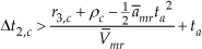
To obtain the region sizes, we need to know the worst-case for a robot avoiding this obstacle. As shown in Figure 4a, the robot approaches the obstacle with a velocity V _mr . It is clear that its velocity component V_mr,t (i.e., tangential to the boundary of the Minkowski sum area) will not cause a collision and it will help the robot to detour around the obstacle. The other component V_mr,n may cause a collision. The worst-case occurs when γ _mr =0 and V_mrn = V̄ _mr . For this case, stopping the robot before contact occurs requires:

${\stackrel{⌢}{r}}_{3,po}={\bar{\delta }}_{r1}$

(22)

$r_{3,po}>{\stackrel{⌢}{r}}_{3,po}+{\rho }_r$

(23)

where ${\stackrel{⌢}{r}}_{3,po}$ is the stopping distance and ${\bar{\delta }}_{r1}$ is given by (3). So ${ℂ}_{3,po}$ may be obtained by Minkowski summation of the obstacle model and disk Π with a radius of r_3,po, as shown in Figure 4b.

For the active region and a holonomic robot similar to (19), we require:

${\stackrel{⌢}{r}}_{2,po}>{\bar{\delta }}_{rx2,po}$

(24)

${\bar{\delta }}_{rx2,po}={\bar{V}}_{mr}\cdot \left(\mathrm{\Delta }{t}_{2,po}+T_s\right)$

(25)

Δt_2,rect must satisfy:

${\bar{V}}_{mr}\cdot \left(\mathrm{\Delta }{t}_{2,po}-t_a\right)+\frac{1}{2}{\bar{a}}_{mr}{t}_a^2>r_{3,po}+B$

(26)

where B is the distance between the robot's position and the boundary of the obstacle in the V_mr,t direction. For the worst-case of B = ½B_len, similar to (21), Δt_2,po must satisfy:

$\mathrm{\Delta }{t}_{2,po}>\frac{r_{3,po}+\frac{1}{2}{B}_{len}-\frac{1}{2}{\bar{a}}_{mr}{t}_a^2}{{\bar{V}}_{mr}}+t_a$

(27)

The corresponding worst-case value of ${\stackrel{⌢}{r}}_{2,po}$ is termed r_2,po. If the robot is nonholonomic then r_2,po should be increased by V̄_mrt_turn. ${\bar{V}}_{mr}{t}_{turn}.{ℂ}_{2,po}$ may then be obtained by Minkowski summation of the obstacle model and disk Π₃ with a circle of radius r_2,po, as shown in Figure 4b.

This can be easily extended to convex and non-convex polygonal obstacles. In the convex case:

1. Enclose the polygon in a minimal area bounding rectangle.

2. Calculate r_2,po and r_3,po for the bounding rectangle.

3. ${ℂ}_{2,po}$ and ${ℂ}_{3,po}$ equal the Minkowski summations of the polygon with disks Π₂ and Π₃, respectively.

An example of this procedure is shown in Figure 5.

Figure 5.

Region design example for a convex polygonal obstacle. (a) Obstacle with its bounding rectangle. (b) Designed regions.

For non-convex polygonal obstacles, the polygon must first be decomposed into convex pieces. The regions are then created for each piece. If the robot enters the active regions of two or more pieces then the virtual forces from those pieces are summed. An example of a U-shaped obstacle will be presented in Section 4.

3. Design of the QVFF virtual force functions

This section begins by discussing the case of a robot avoiding a single human. The geometric configuration of the goal, the robot and the human is presented in Figure 6. We assume that the robot goal is stationary and outside of the active region(s) of the obstacle(s) for safety. In this figure, P _g , P _r and P _h are the current position vectors of the goal, the robot and the human, respectively. V _mr and V _h are the velocity vectors of the robot and the human. We have:

Figure 6.

Example of the attractive, repulsive and detour forces when avoiding a human.

$E=P_g-P_r,$

(28)

$D=P_r-P_h \text{and}$

(29)

$W=P_g-P_h$

(30)

where E is the vector from the robot to its goal, D is the vector from the obstacle to the robot and W is the vector from the obstacle to the goal.

An attractive virtual force is used to guide the robot to the goal. It is activated when the robot is within ${ℂ}_1$ or ${ℂ}_2$ . Its force function is defined as:

$F_a=\{\begin{array}{ccc}{K}_{1}E+K_2\stackrel{.}{E}& & \text{if}{P}_r\in {ℂ}_2\cup {ℂ}_1\\ \text{undefined}& & \text{if}{P}_r\in {ℂ}_3\end{array}$

(31)

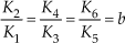
where K₁ and K₂ are the positive attractive virtual force gains.

A repulsive virtual force is used to keep the robot away from the human and is activated when the robot is within ${ℂ}_2$ . The repulsive force is normally a function of the distance between the human and robot. We use the closest distance² d = ‖D‖₂ - ρ_r - ρ_h and its rate of changed. Its direction is along D. Note that when d ≤ 0 a collision has occurred. If we define d ₂ = d - r₂ + ρ _r and d₃ = d - r₃ + ρ _r then $d_2\le 0\wedge d_3\ge 0\iff P_r\in {ℂ}_2$ and $d_3<0\iff P_r\in {ℂ}_3$ . We propose the new repulsive force function:

$F_{\mathrm{\Lambda }}=\{\begin{array}{ccc}\left(K_3\mathrm{\Lambda }+K_4{\stackrel{.}{\mathrm{\Lambda }}}^{*}\right)u_{\mathrm{\Lambda }}& & \text{if}{P}_r\in {ℂ}_2\\ \text{undefined}& & \text{if}{P}_r\in {ℂ}_1 \cup {ℂ}_3\end{array}$

(32)

where K₃ and K₄ are the positive repulsive force gains, u_Ais a unit vector along D, pointing away from the human, $\mathrm{\Lambda }=\frac{d_2{}^2}{d_3}$ and ${\stackrel{.}{\mathrm{\Lambda }}}^{*}=-\stackrel{.}{d}\frac{d_2{}^2}{d_3{}^2}=-{\kappa }_{\mathrm{\Lambda }}\stackrel{.}{d}$ . Note that $P_r\in {ℂ}_2\iff r_3<d<r_2$

The numerator term of λ, d₂² causes the repulsive force to gradually increase from zero when the robot enters the active region. The denominators, d₃ and d₃², cause the force to increase greatly when the robot is near the boundary of ${ℂ}_3$ . This is useful for avoiding multiple obstacles. When the robot is pushed close to ${ℂ}_3$ by another obstacle, the repulsive force from this obstacle is significantly increased. This tends to push the robot away from ${ℂ}_3$ of the obstacle. Note that the velocities of the human and robot are included in ${\stackrel{.}{\mathrm{\Lambda }}}^{*}$ of (32). When the human and robot approach each other ḋ<0, so ${\stackrel{.}{\mathrm{\Lambda }}}^{*}>0$ and the repulsive force will increase to push the robot away.

The detour force, F_Ψ, is a virtual force perpendicular to D. Its main purpose is to push the robot to detour around the human while still moving to the goal. Its other purpose is dealing with the collinear condition. The first issue when designing this force is selecting its sense. This issue has not been adequately addressed in the existing literature. In Figure 6, the two possible senses for F_Ψ are labelled F_Ψ and F_Ψ. If the sense of the force was F_Ψ the robot would try to pass in front of the obstacle. This is acceptable for stationary obstacles, but is not desirable with humans for physical and emotional reasons, as was discussed in Section 1.1. So the sense of F_Ψ* is the correct choice. Figure 7 shows the correct sense of Fin relation to the kinematics of the robot and human. In Figure 7a, the goal and robot are on different sides of the human's velocity line. In this case, the detour force should cause the robot to detour around behind the human to prevent blocking the human. In Figure 7b, since the goal and robot are on the same side of the human's velocity line, the robot will not block the human. Then, the sense of F_Ψ should point it towards the goal to help the robot reach its goal faster. For the collinear condition, since the robot, its goal, and the obstacle are collinear and their velocity lines are also along this line, the condition for avoidance is symmetrical to this line. When there are other obstacles, we should choose the sense that satisfies $u_{\psi }\cdot {\displaystyle \sum F_{\psi ,i}}>0$ , where ${\displaystyle \sum F_{\psi ,i}}$ is the sum of the detour forces from the other obstacles and u_Ψ is the unit vector in the direction of the detour force. This force should be zero when the robot is between the goal and the human (i.e., when α = β). Furthermore, since they produce no velocity line, the sense of u_Ψ should be towards the goal with stationary obstacles to reach the goal earlier. So, we propose the new detour force function:

Figure 7.

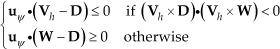
Determination of the correct sense of the detour force.

$F_{\psi }=\{\begin{array}{ccc}\left(K_5\psi +K_6{\stackrel{.}{\psi }}^{*}\right)u_{\psi }& & \text{if}{P}_r\in {ℂ}_2\\ \text{undefined}& & \text{if}{P}_r\in {ℂ}_1\cup {ℂ}_3\end{array}$

(33)

where K₅andK₆ are the positive detour force gains, Ψ=d²₂Φ,Φ=α-β and Ψ=d²₂Φ. The sense of u_Ψ should be chosen to satisfy:

$\{\begin{array}{l}{u}_{\psi }\bullet \left(V_h-D\right)\le 0\text{ if }\left(V_h\times D\right)\bullet \left(V_h\times W\right)<0\\ u_{\psi }\bullet \left(W-D\right)\ge 0\text{ otherwise}\end{array}$

(34)

To ensure stability, we add the following stabilizing virtual force into the VFF:

$F_L=\{\begin{array}{cc}\frac{K_L{u}_L}{{\Vert v_L\Vert }_2}& \text{if}{P}_r\in {ℂ}_2\\ \text{undefined}& \text{if}{P}_r\in {ℂ}_1\cup {ℂ}_3\end{array}$

(35)

where $v_L=K_1\stackrel{.}{E}+K_3{\stackrel{.}{\mathrm{\Lambda }}}^{*}{u}_{\mathrm{\Lambda }}+K_5{\stackrel{.}{\psi }}^{*}{u}_{\psi }$ , $u_L$ is a unit vector in the direction of v _L ,

$\begin{array}{l}{K}_L=\{\begin{array}{cc}\mathrm{\Omega }& \mathrm{\Omega }>0\\ 0& \mathrm{\Omega }\le 0\end{array},\\ \mathrm{\Omega }=-K_1{\stackrel{.}{E}}^{\mathrm{T}}\left(K_3\mathrm{\Lambda }{u}_{\mathrm{\Lambda }}+K_5\psi u_{\psi }\right)-K_3^2\frac{2\stackrel{.}{d}{d}_2}{d_3}\mathrm{\Lambda }+\frac{1}{2}{M}_r{K}_3{\stackrel{.}{\kappa }}_{\mathrm{\Lambda }}{\stackrel{.}{d}}^2+\\ \hspace{1em}\hspace{1em}{K}_5{\stackrel{.}{\psi }}^{*}\left(a_o^{\mathrm{T}}{u}_{\psi }-K_1{E}^{\mathrm{T}}{u}_{\psi }\right)-K_3\stackrel{.}{\mathrm{\Lambda }}\left(K_1{E}^{\mathrm{T}}{u}_{\mathrm{\Lambda }}-a_o^{\mathrm{T}}{u}_{\mathrm{\Lambda }}\right)+\\ \hspace{1em}\hspace{1em}\frac{1}{2}{M}_r{K}_5{d}_2{}^2\stackrel{.}{d}{\stackrel{.}{\mathrm{\Phi }}}^2-M_r{K}_5{d}_{2}d\stackrel{.}{d}{\stackrel{.}{\mathrm{\Phi }}}^2-K_5^2{d}_2\stackrel{.}{d}{\mathrm{\Phi }}^2\end{array}$

and M_r is the virtual mass of the robot.

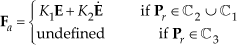
Our VFF is a combination of the four forces and is termed quad-VFF (QVFF). Thus, the QVFF for the robot with a single human/obstacle is:

$F_V=\{\begin{array}{ccc}{F}_a& & \text{if}{P}_r\in {ℂ}_1\\ \begin{array}{l}{F}_a+F_{\mathrm{\Lambda }}+F_{\psi }+F_L\\ \text{ undefined}\end{array}& & \begin{array}{l}\text{if}{P}_r\in {ℂ}_2\\ \text{if}{P}_r\in {ℂ}_3\end{array}\end{array}$

(36)

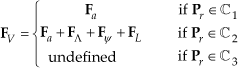
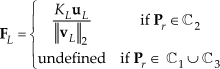
If the robot intrudes into ${ℂ}_3$ , since it may not have enough space for collision avoidance, the VFF is not used and the robot is decelerated to a stop. This stopping action should prevent or at least mitigate the collision. Any other action made by the robot could worsen the situation.

A VFF should be continuous in order to reduce path oscillations. For the QVFF to be continuous the virtual forces at the boundary between ${ℂ}_1$ and ${ℂ}_2$ must be equal. From (31) and (36), at the boundary of ${ℂ}_1$ we have:

$F_{V,P_r\in {ℂ}_1}=K_{1}E+K_2\stackrel{.}{E}$

(37)

From (32)–(36), at the outer boundary of ${ℂ}_2$ we have:

$\underset{d_2\to 0}{\lim }\mathrm{\Lambda }=\underset{d_2\to 0}{\lim }{d}_2{}^2∕d_3=0,$

(38)

$\underset{d_2\to 0}{\lim }{\stackrel{.}{\mathrm{\Lambda }}}^{*}=\underset{d_2\to 0}{\lim }-\stackrel{.}{d}{d}_2{}^2∕d_3{}^2=0,$

(39)

$\underset{d_2\to 0}{\lim }\psi =\underset{d_2\to 0}{\lim }{d}_2{}^2\mathrm{\Phi }=0 \text{and}$

(40)

$\underset{d_2\to 0}{\lim }{\stackrel{.}{\psi }}^{*}=\underset{d_2\to 0}{\lim }{d}_2{}^2\stackrel{.}{\mathrm{\Phi }}=0$

(41)

From (38)–(41) it follows that:

$\underset{d_2\to 0}{\lim }{F}_{\mathrm{\Lambda }}=\underset{d_2\to 0}{\lim }{F}_{\psi }=\underset{d_2\to 0}{\lim }{F}_L=0$

(42)

Therefore:

$\underset{d_2\to 0}{\lim }{F}_{V,P_r\in {ℂ}_2}=K_{1}E+b{K}_1\stackrel{.}{E}=F_{V,P_r\in {ℂ}_1}$

(43)

From (43) the piecewise QVFF is continuous.

Extending the above analysis, if the robot is sharing its environment with N static or dynamic obstacles (which could include other robots), the force field will be:

$F_V=\{\begin{array}{cc}\begin{array}{c}{F}_a\\ \text{undefined}\end{array}& \begin{array}{c}\text{if}{P}_r\in {ℂ}_1\\ \text{if}{P}_r\in {ℂ}_{3,i}i\in [1,...,N]\end{array}\\ F_a+{\displaystyle \sum _{i=1}^N{c}_i\left(F_{\mathrm{\Lambda },i}+F_{\psi ,i}\right)+F_L}& \text{otherwise}\end{array}$

(44)

where $c_i=\{\begin{array}{cc}1& \text{if}{P}_r\in {ℂ}_{2,i}\\ 0& \text{otherwise}\end{array}$ , $F_{\mathrm{\Lambda },i}$ , and F_Ψ,i are the repulsive and detour forces for the i^th obstacle, respectively, $v_L=K_1\stackrel{.}{E}+{\displaystyle \sum _{i=1}^N{c}_i\left(K_{3,i}{\stackrel{.}{\mathrm{\Lambda }}}_i^{*}{u}_{\mathrm{\Lambda },i}+K_{5,i}{\stackrel{.}{\psi }}_i^{*}{u}_{\psi ,i}\right)}$ , $F_L=\frac{K_L{u}_L}{{\Vert v_L\Vert }_2}$ and $u_L$ is the unit vector along the direction of v _L . With (44), the QVFF is again piecewise. It is also continuous. Proof is given in [24] and is omitted here for brevity.

4. Stability analysis of the QVFF

As mentioned in Section 1.2, with VFF-based algorithms the desired acceleration of the robot is obtained by dividing F _v by M_r and the desired velocity may be obtained by Euler integration. Assuming the robot can track the desired motion trajectory, stability of the QVFF implies stability of the robot motion. Our stability analysis is based on Lyapunov's second method. We will start the stability analysis for the navigation condition with only one static or dynamic obstacle. From (36), when the robot is inside ${ℂ}_1$ , F _v only depends on E and Ė, so the state vector is X₁ = [E^T E^T]^T. When X₁ = 0 the robot is stopped at its goal. When the robot is inside ${ℂ}_2$ , the QVFF state vector is $X_2={\left[\begin{array}{cccccc}{E}^{\mathrm{T}}& {\stackrel{.}{E}}^{\mathrm{T}}& \mathrm{\Lambda }& {\stackrel{.}{\mathrm{\Lambda }}}^{*}& \psi & {\stackrel{.}{\psi }}^{*}\end{array}\right]}^{\mathrm{T}}$ . The piecewise Lyapunov function candidate for the QVFF is:

$V=\{\begin{array}{ccc}{V}_1=\frac{1}{2}{X}_1^{\mathrm{T}}{Q}_1{X}_1,& & \text{if }{P}_r\in {ℂ}_1\\ V_2=\frac{1}{2}{X}_2^{\mathrm{T}}{Q}_2(d)X_2,& & \text{if }{P}_r\in {ℂ}_2\end{array}$

(45)

where $Q_1=\left[\begin{array}{cccc}{K}_1^2& K_1^2& M_r{K}_1& M_r{K}_1\end{array}\right]\cdot I_4,\hspace{1em}\hspace{1em}\hspace{1em}\hspace{1em}\hspace{1em}\hspace{1em}\hspace{1em}$ $Q_2(d)=\left[\begin{array}{cccccccc}{K}_1^2& K_1^2& M_r{K}_1& M_r{K}_1& K_3^2& h_{\mathrm{\Lambda }}& K_5^2& h_{\psi }\end{array}\right]\cdot I_8$ , $h_{\mathrm{\Lambda }}=M_r{K}_3\frac{d_3{}^2}{d_2{}^2}$ and $h_{\psi }=M_r{K}_5\frac{d}{d_2{}^2}$ . Note that when the robot is inside ${ℂ}_3$ the robot is commanded to stop. V₁ and V₂ are clearly positive definites. A piecewise Lyapunov function candidate must be continuous to be valid. To check the continuity of V at the boundary between $V_1$ and $V_2$ :

$\underset{d\to r_2}{\lim }{V}_2=\frac{1}{2}{K}_1^2{E}^{\mathrm{T}}E+\frac{1}{2}{M}_r{K}_1{\stackrel{.}{E}}^{\mathrm{T}}\stackrel{.}{E}$

(46)

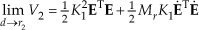
Therefore:

$\underset{d\to r_2}{\lim }{V}_{2,P_r\in {ℂ}_2}=V_{1,P_r\in {ℂ}_1},$

(47)

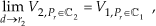
and the continuity is proven.

When $P_r\in {ℂ}_1$ , from (31) and (44) we observe that $F_{V,P_r\in {ℂ}_1}$ has the same form as proportional plus derivative control. It is straightforward to prove that the QVFF is locally asymptotically stable at the goal, subject to the condition $F_{V,P_r\in {ℂ}_1}$ . The details are omitted here for brevity and are provided in [24].

When $P_r\in {ℂ}_2$ , if we set:

$\frac{K_2}{K_1}=\frac{K_4}{K_3}=\frac{K_6}{K_5}=b$

(48)

where b > 0, then the first derivative of V₂ is:

${\stackrel{.}{V}}_2=\{\begin{array}{cc}-b{\Vert v_L\Vert }_2^2& \mathrm{\Omega }>0\\ -b{\Vert v_L\Vert }_2^2+\mathrm{\Omega }& \mathrm{\Omega }\le 0\end{array}$

(49)

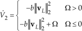
From (49) it is clear that:

${\stackrel{.}{V}}_2\le -b{\Vert v_L\Vert }_2^2\le 0$

(50)

When $P_r\in {ℂ}_2$ , according to (50), V₂≤0. As shown in [24], V̇₂=0 and ${\stackrel{.}{P}}_h=0$ simultaneously. This is clearly unlikely. When V̇₂<0 the QVFF will drive the robot out of ${ℂ}_2$ and into ${ℂ}_1$ . When it is inside ${ℂ}_1$ the robot will asymptotically reach the goal as described above.

The stability analysis can also be expanded to include multiple static or dynamic obstacles. If the robot is in the active region of N obstacles, the VFF state for V₂ is:

${\mathbf{X}}_2={[{\mathbf{E}}^{\mathrm{T}}{\stackrel{.}{\mathbf{E}}}^{\mathrm{T}}{\mathrm{\Lambda }}_1{\stackrel{.}{\mathrm{\Lambda }}}_1^{\ast }{\psi }_1{\stackrel{.}{\psi }}_1^{\ast }\dots {\mathrm{\Lambda }}_N{\stackrel{.}{\mathrm{\Lambda }}}_N^{\ast }{\psi }_N{\stackrel{.}{\psi }}_N^{\ast }]}^{\mathrm{T}}$

(51)

and Q₂(d) becomes:

$\begin{array}{l}{Q}_2(d)=[\begin{array}{ccccccccc}{K}_1^2& K_1^2& M_r{K}_1& M_r{K}_1& K_{3,1}^2& h_{\mathrm{\Lambda },1}& K_{5,1}^2& h_{\psi ,1}& \dots \end{array}\\ {\begin{array}{cccc}\hspace{1em}\hspace{1em}{K}_{3,N}^2& h_{\mathrm{\Lambda },N}& K_{5,N}^2& h_{\psi ,N}\end{array}]}^{\mathrm{T}}{I}_{4N+4}\end{array}$

(52)

Then we can use (45) to build the Lyapunov function for N obstacles. This function for N obstacles is continuous, since ${\mathrm{\Lambda }}_i$ , ${\stackrel{.}{\mathrm{\Lambda }}}_i^{*}$ , ${\psi }_i$ and ${\stackrel{.}{\psi }}_i^{*}$ for i = 1,…, N equal zero at the edge of the active region of all N obstacles. We can see that if the robot comes into the active region of another obstacle, the value of N in (51) and (52) will be increased to N+1. Since ${\mathrm{\Lambda }}_{N+1}$ , ${\stackrel{.}{\mathrm{\Lambda }}}_{N+1}^{*}$ , ${\psi }_{N+1}$ and ${\stackrel{.}{\psi }}_{N+1}^{*}$ equal zero at the edge of the active region of the N+1 obstacle, V₂ is still continuous. The Lyapunov function for N+1 obstacles is also continuous and the stability analysis can be performed using the same approach as in the single obstacle case. Therefore, arbitrary numbers of obstacles can be included in the stability analysis. Furthermore, it can be shown that the same stability conclusions from the single obstacle case apply to the multiple obstacle case, except that V̇₂ = 0 is more likely to occur. Detailed proof is given in [24] and is omitted here for brevity. The V̇₂ =0 case is more likely to occur than with a single obstacle due to the interaction of the virtual forces with the obstacles. The corresponding equilibrium point is termed a “local minima” point in the robot collision avoidance literature (e.g., [14, 19]). This is particularly a problem with stationary obstacles since the robot will be prevented from reaching its goal indefinitely. However, local minima can often be prevented by using large values of K₅ and K₆ to create a large detour force. An example is shown in Figure 8. The robot starts inside the U-shaped obstacle. The obstacle has been decomposed into three rectangular obstacles whose regions were calculated as described in Section 2.5. Initially, $P_r\in {ℂ}_1$ , $F_V=F_a$ and the robot is driven straight towards its goal. It next enters ${ℂ}_2$ . While $P_r\in {ℂ}_2$ , $F_V$ is dominated by the repulsive and detour forces. F_Ψ keeps it outside of ${ℂ}_3$ , while $F_{\mathrm{\Lambda }}$ drags it around the obstacle. Finally it is pulled out of ${ℂ}_2$ and to the goal by F _a .

Figure 8.

Simulation of the QVFF algorithm with a holonomic robot and a U-shaped obstacle.

5. Results and discussion

5.1 Experimental Hardware

A differential-drive nonholonomic robot and vision system was built for experimental verification of our algorithm. A bottom view of the robot is shown in Figure 9. Wheels 1 and 2 are driven by DC motors via a 10:1 worm gear. Wheel 3 is a passive omni-directional wheel that prevents the robot from tipping. The wheel positions are measured by optical encoders. The encoder data and motor voltages are transmitted to/from a PC-based controller using an umbilical cable. The experimental setup also includes a calibrated colour video camera for capturing images of the human and the robot. Colour patches are attached to the human's shoulder and the robot at known Z heights, as shown in Figure 10. With a standard PC, the X-Y positions of the robot and the X position of the human are estimated from the image centroids of the colour patches using the camera calibration matrix and the patch heights. Note that the low ceiling height in our laboratory prevented the camera from being placed overhead. Due to the camera's location and the human's shoulder height, the accuracy of the Y position estimates is very poor, so only the human's X position estimates are used. The velocities of the robot and the human are calculated by backward differencing their estimated positions. The experimental hardware has a sampling period of T_s = 0.06 s. Unfortunately, it is only possible to reliably track one human with our setup since the colour patch on the 2^nd human could be occluded by the body of the 1^st human. Further details on this hardware are provided in [24].

Figure 9.

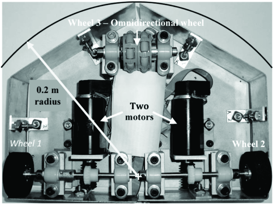
The nonholonomic robot used in the experiments.

Figure 10.

Captured image of the robot avoiding a walking human. The red, green and yellow colour patches are used for position tracking.

5.2 Avoiding a walking human in the collinear condition

As explained in Sections 1.2 and 2.3, the collinear condition is the worst-case for a robot and a single moving obstacle. Simulation and experimental results for a walking human and nonholonomic and holonomic mobile robots in the collinear condition are shown in Figure 11. The robots both have a radius of ρr = 0.2 m, a maximum velocity of V̄ _mr =0.7 m/s and maximum acceleration of ā _mr = 10 m/s². The maximum angular acceleration of the nonholonomic robot is $\overline{\stackrel{.}{\omega }}=70{\text{rad/s}}^2$ . The maximum human velocity was assumed to be V̄ _h = 1 m/s [23]. Substituting these values and the ρ _h value from Section 2.2 into our region sizing equations (Sections 2.2 and 2.3) we obtained r_2,nh = 2.1m and r_3,nh = 0.4m for the nonholonomic robot and r₂ = 1.7m and r₃ = 0.4m for the holonomic robot. The human starts from position (0.1, 0.6)m, moves from left to right and stops at (4, 0.6)m. At the same time, the robot starts from (4, 0.6)m and moves from right to left towards its goal at (0, 0.6)m. From Figure 11 we can see that the simulation and experimental results for the nonholonomic robot are similar. The discrepancy is mainly due to wheel slip. In comparison to the simulation with the holonomic robot, we can see that the nonholonomic robot moves away from the goal (i.e., in the positive X-direction) more than the holonomic robot. The time required for the nonholonomic robot to turn to avoid the human allowed d to decrease further as the human approached. This caused a larger repulsive force that pushed the robot farther from the goal. This is apparent in the plots of e and the robot path. The d values are always positive, demonstrating that no collision occurred. Furthermore, the d and e plots show that the holonomic robot was safer (since its minimum d was larger) and arrived at the goal 24% sooner than the nonholonomic robot. Note that the measured human position and velocity data were used in the computer simulations. As explained in section 5.1, our hardware can only track one human's motion in the X direction. Since we wanted to evaluate the performance of the QVFF for more challenging environments we simulated more complex human motions to obtain the results presented in the following sections.

Figure 11.

Experimental and simulation results for nonholonomic and holonomic robots navigated by the QVFF algorithm, with a human walking in the collinear condition. (a) Paths. (b) Human velocity. (c) Closest distances to the human. (d) Distances to the goal.

5.3 Comparison with five state-of-the-art navigation algorithms

In this section simulations with five state-of-the-art navigation algorithms for moving obstacles are compared with the QVFF algorithm. The human and robot paths, the closest distance from the robot to the human and the distance from the robot centre to the goal are plotted for the six algorithms in Figure 12. A human path with an unpredictable direction change is used (plotted in light green). The robot is holonomic with the same specifications as used in the previous section.

The robot starts from (4, 0)m and must avoid the walking human to reach its goal at (0, 0)m. The walking human initially starts from (0.6, 0)m with a (1, 0)m/s velocity. After 1s, the human slows down with a (−1, 0)m/s² deceleration until it stops at (2, 0)m and then moves sideways with a (0, 1)m/s² acceleration. After the human's velocity reaches (0, 1)m/s, the human maintains a constant velocity. In the figure, VO denotes the velocity obstacle algorithm [2], RRT denotes the rapidly exploring random trees algorithm [15], D* denotes the D* algorithm [6], Ge & Cui denotes their algorithm [13] and Masoud denotes his algorithm [14]. The gains for the Masoud, Ge & Cui and QVFF algorithms were optimally tuned. The detailed tuning process is omitted here for brevity and can be found in [24]. The first three algorithms (i.e., VO, D* and RRT) belong to the first category described in Section 1.2, while the remainder belong to the second category. During the simulations, the future motion of the human, including the walking direction change, is unknown for all six algorithms. From Figure 12b we can see that the first three algorithms caused collisions (indicated by d reaching zero) after the human changed its motion direction. These collisions occurred at the locations shown by the asterisks in Figure 12a. The algorithms in the second category all successfully completed the navigation. The robot path with the Ge & Cui algorithm ran straight from the robot start position to its goal. It was not plotted to avoid obscuring the human's path. It did not detour around the human since their detour force is zero under the collinear condition. As shown by the e plot, their repulsive force caused the robot to stop momentarily at 1.9s and then move backwards until the time reached 4.1s.

Figure 12.

Comparison of simulation results for six navigation algorithms avoiding a human with unpredictable motion. (a) Paths. (b) Closest distances between the robot and humans. (c) Distance from the robot centre to the goal.

After that, the motion of the human in the positive Y direction allowed their algorithm to drive the robot to the goal. It arrived at 10.9s. Of course this “backup and wait” strategy would prevent the robot from reaching the goal if the obstacle was static. The Masoud and QVFF algorithms made detours to avoid the human. With the QVFF algorithm the minimum d was 0.8m and the robot reached the goal at 10.2s. The larger detour made by the Masoud algorithm increased its minimum d to 1.2m, but also increased its arrival time to 14.0s.

5.4 Collision avoidance with three walking humans

The QVFF algorithm was also simulated with an environment containing three walking humans (denoted Human 1, Human 2 and Human 3). The paths of the humans and robot are plotted in Figure 13a.

Figure 13.

Simulation of the QVFF algorithm for an environment with three walking humans. (a) Paths. (b) Closest distances between the robot and humans. (c) Distance from the robot centre to the goal.

The closest distances from the robot to each human are plotted in Figure 13b and the distance from the robot centre to the goal is plotted in Figure 13c. The robot was identical to the previous section. It started from (3.85, 0.6)m and its goal was at (0, 0.6)m. The motion of Human 1 was unpredictable. Starting from (0.6, 0.6)m, he moved to the right at 0.7m/s velocity. After 1.4s, he smoothly turned counter-clockwise until the time equalled 4.4s. Next, he stopped for 1.0s. Finally, he moved left and downwards at 1m/s. Simultaneously, Human 2 started from (0, 0)m and moved left at 1m/s and Human 3 started from (1.5, −4.5)m and moved upwards at 1m/s velocity. From Figure 13b we can see that the robot successfully avoided all three humans. The minimum d was 0.22m to Human 1. This is not surprising since his motion was the most unpredictable. The robot arrived at its goal in 14.2s.

6. Conclusions

A novel VFF-based navigation algorithm, termed QVFF, was presented. It is primarily intended for mobile robots sharing working environments with people. It features improved virtual force functions for avoiding moving obstacles, it may be used with both holonomic and nonholonomic robots and its stability was proven using Lyapunov's second method. Active and critical regions were used to deal with the uncertainty of human motion. A procedure was introduced to calculate the region sizes for disk-shaped and polygonal obstacles based on the worst-case avoidance conditions. Simulation and experimental results were presented. The QVFF algorithm outperformed five state-of-the-art navigation algorithms for an environment with one human walking with an unpredictable change in direction. For a human walking in the collinear condition and a challenging environment containing three walking humans, the QVFF algorithm successfully generated collision-free paths to the goal.