Sage Journals: Discover world-class research

Abstract

This paper develops a robust adaptive control for a class of nonlinear systems using the backstepping method. The proposed robust adaptive control is a recursive method based on the Lyapunov synthesis approach. It ensures that, for any initial conditions, all the signals of the closed-loop system are regularly bounded and the tracking errors converge to zero. The results are illustrated with simulation examples.

Keywords

Robust Adaptive Control System Nonlinear Systems Backstepping Method Closed-Loop States

1. Introduction

In recent decades, a large number of papers have studied the problem of robust adaptive control of nonlinear systems (see, e.g., [1 -15] and references therein). In [1], a new adaptive law based on an optimal control formulation for the minimization of the L₂ norm of the tracking bounded error is considered. A method for designing a global adaptive neural network controller for a class of uncertain non-linear systems is proposed in [2]. In [3 -9], adaptive control of uncertain nonlinear systems using backstepping is developed. In these papers, the backstepping method guarantees global stabilities, tracking and transient performance for a broad class of strict-feedback system. New adaptive feedforward cancellations (AFC) control providing periodic tracking and/or periodic disturbance rejection is proposed in [10]. In [11], a robust control system combining backstepping and sliding mode control techniques is used to realize the synchronization of two gap junction coupled chaotic FitzHugh–Nagumo (FHN) neurons in the external electrical stimulation. The paper [12] introduces an optimal H_∞ adaptive PID (OHAPID) control scheme for a class of nonlinear chaotic system with uncertainties and external disturbances. In [13], an adaptive backstepping control scheme is proposed for task-space trajectory tracking of robot manipulators. In [14], an adaptive integral backstepping algorithm is proposed as a means to effectuate the attitude control of a 3-DOF helicopter. In [15], a backstepping approach is used for the design of a discontinuous state feedback controller for the controller.

The main contribution of this paper is the design of an adaptive backstepping control method for a class of uncertain single input single output nonlinear systems which can be transformed into a triangular form. Many systems, such as AC motors, spacecraft, magnetic suspension and robot manipulators, possess this structure [14]. These systems can be built from subsystems that can be stabilized [14, 15]. In this paper, we assume that the bounds of the uncertainty system parameters are available. The adaptive calculating procedure of the control is a recursive procedure based on the Lyapunov approach. It is composed of several steps. It can start at the known-stable system and back out new controllers that gradually stabilize each outer subsystem. The procedure stops when the final external control is reached. Compared with the adaptive control scheme, the proposed control approach has the advantages of adaptive technique and robust control, which makes this approach attractive for a wide class of nonlinear systems with both uncertain nonlinearities and disturbances.

This paper is organized as follows: the formulation of the problem is introduced in Section 2; the controller design and stability analysis are presented in Section 3; the results of the simulation, illustrating the efficiency of the proposed controller, are presented in Section 4.

2. Problem statement and preliminaries

Let us consider the following nonlinear system

{\begin{matrix} {\dot{x}}_{i} = h_{i} ({\bar{x}}_{i}) + φ_{i} ({\bar{x}}_{i}) x_{i + 1} + Δ_{i} ({\bar{x}}_{i}), i = 1, \dots, n - 1 \\ {\dot{x}}_{n} = h_{n} ({\bar{x}}_{n}) + φ_{n} ({\bar{x}}_{n}) u + Δ_{n} ({\bar{x}}_{n}) \\ y = x_{1} \end{matrix}

(1)

where: x̄_i = [x₁,…,x_i]^T ∈ ℝⁱ is the state of the i-th subsystem; x̄_n = [x₁,…,x_n]^T ∈ ℝⁿ, u ∈ ℝ and y ∈ ℝ are the state, the input and the output of the overall system, respectively; h_i(x̄_i) ∈ ℝ, i = 1,…,n are the known functions; Δ_i(x̄_i) are unknown Lipschitz continuous functions such that:

{\begin{matrix} | Δ_{i} ({\bar{x}}_{i}) | \leq l_{i}, l_{i} \geq 0 \\ \forall {\bar{x}}_{i} \in ℝ^{i}, i = 1, \dots, n \end{matrix}

(2)

where: l_i are known constants.

The known functions φ_i(x̄_i) ∈ ℝ are defined as

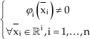
{\begin{matrix} φ_{i} ({\bar{x}}_{i}) \neq 0 \\ \forall {\bar{x}}_{i} \in ℝ^{i}, i = 1, \dots, n \end{matrix}

(3)

The purpose of this paper is the design of a control u that ensures the tracking output y sticks to a specified trajectory y_d ∈ ℝ so that all system variables are bounded.

The desired reference signal y_d(t) is of class C^∞, t ≥ 0 well as y_d, ẏ_d,…, y_d^(n-1), y_d⁽ⁿ⁾ are known and bounded. The tracking error is defined as

e = y_{d} - y

(4)

The determination procedure of the control u is presented in the next section.

3. Robust adaptive controller design and stability analysis

The control u is calculated using the backstepping method. The calculation procedure involves n steps. From step 1 to stepn-1, the virtual control inputs γ_i, = 1,…,n-1 are designed, respectively. The practice control input u is built at step n. The detailed design is described in the following steps [3 -9, 11, 13 -15].

Step 1: In this step, the design objective is to choose the virtual controller γ₁ so that the tracking error λ₁ = -e = x₁ – y_d is as small as possible. The time derivative of λ₁ is

{\dot{λ}}_{1} = {\dot{x}}_{1} - {\dot{y}}_{d} = h_{1} (x_{1}) + φ_{1} (x_{1}) x_{2} - {\dot{y}}_{d} + Δ_{1} (x_{1})

(5)

Introducing the variable:

λ_{2} = x_{2} - γ_{1} (x_{1}, c_{1}) - {\dot{y}}_{d}

(6)

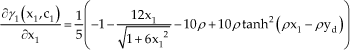
We then choose:

γ_{1} (x_{1}, c_{1}) = \frac{1}{φ_{1} (x_{1})} (- c_{1} λ_{1} - h_{1} (x_{1}) - φ_{1} (x_{1}) {\dot{y}}_{d} + {\dot{y}}_{d} - l_{1} sgn (λ_{1}))

(7)

where:

sgn (λ_{1}) = {\begin{matrix} 1 i f λ_{1} > 0 \\ 0 i f λ_{1} = 0 \\ - 1 i f λ_{1} < 0 \end{matrix}

(8)

The parameter c₁ ∈ ℝ is selected such that c₁ > 0.

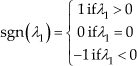
For p ≫ 1, a smooth approximation of the sgn function is

sgn (λ_{1}) \approx \tanh (ρ λ_{1})

(9)

The relationship (9) is usually used to reduce the chattering which is caused by the sgn function [16].

Therefore, the equation (7) can be written in the following form

γ_{1} (x_{1}, c_{1}) = \frac{1}{φ_{1} (x_{1})} (- c_{1} λ_{1} - h_{1} (x_{1}) - φ_{1} (x_{1}) {\dot{y}}_{d} + {\dot{y}}_{d} - l_{1} \tanh (ρ λ_{1}))

(10)

Consider the following Lyapunov function candidate

V_{1} = \frac{1}{2} λ_{1}^{2}

(11)

By using (1), (5), (6), (9) and (10), the time derivative of V₁ is

{\dot{V}}_{1} = {\dot{λ}}_{1} λ_{1} \leq - c_{1} λ_{1}^{2} + φ_{1} (x_{1}) λ_{1} λ_{2}

(12)

where the coupling term φ₁(x₁)λ₁λ₂ will be cancelled in the next step.

Step i (2≤i≤n-1): Similar to step 1, the virtual controller γ_i will be chosen to make the error variable λ_i = x_i – γ_i-1(x_i-1, c₁,…,c_i-1) – y_d^(i-1) as small as possible. The time derivative of λ₁ is expressed as:

\begin{matrix} {\dot{λ}}_{i} = {\dot{x}}_{i} - {\dot{γ}}_{i - 1} ({\bar{x}}_{i - 1}, c_{1}, \dots, c_{i - 1}) - y_{d}^{(i)} \\ = h_{i} ({\bar{x}}_{i}) + φ_{i} ({\bar{x}}_{i}) x_{i + 1} - y_{d}^{(i)} + Δ_{i} ({\bar{x}}_{i}) \\ - \sum_{j = 1}^{i - 1} \frac{\partial γ_{i - 1} ({\bar{x}}_{i - 1}, c_{1}, \dots, c_{i - 1})}{\partial x_{j}} \\ \times (h_{j} ({\bar{x}}_{j}) + φ_{j} ({\bar{x}}_{j}) x_{j + 1} + Δ_{j} ({\bar{x}}_{j})) \end{matrix}

(13)

The variable λ_i+1 is as follows

λ_{i + 1} = x_{i + 1} - γ_{i} ({\bar{x}}_{i}, c_{1}, \dots, c_{i}) - y_{d}^{(i)}

(14)

{\begin{matrix} \begin{matrix} γ_{i} ({\bar{x}}_{i}, c_{1}, \dots, c_{i}) = \frac{1}{φ_{i} ({\bar{x}}_{i})} (- c_{i} λ_{i} - h_{i} ({\bar{x}}_{i}) - φ_{i} ({\bar{x}}_{i}) y_{d}^{(i)} \\ + \sum_{j = 1}^{i - 1} \frac{\partial γ_{i - 1} ({\bar{x}}_{i - 1}, c_{1}, \dots, c_{i - 1})}{\partial x_{j}} \\ \times (h_{j} ({\bar{x}}_{j}) + φ_{j} ({\bar{x}}_{j}) x_{j + 1} \\ - l_{j} \tanh (ρ λ_{i} \frac{\partial γ_{i - 1} ({\bar{x}}_{i - 1}, c_{1}, \dots, c_{i - 1})}{\partial x_{j}})) \\ + y_{d}^{(i)} - φ_{i - 1} ({\bar{x}}_{i - 1}) λ_{i - 1} - l_{i} \tanh (ρ λ_{i})) \end{matrix} \\ c_{i} > 0 \end{matrix}

(15)

The Lyapunov function candidate is defined as:

V_{i} = V_{i - 1} + \frac{1}{2} λ_{i}^{2}

(16)

Its derivative is:

\begin{array}{l} {\dot{V}}_{i} = {\dot{V}}_{i - 1} + {\dot{λ}}_{i} λ_{i} \\ \leq - \sum_{j = 1}^{i} c_{i} λ_{i}^{2} + φ_{i} ({\bar{x}}_{i}) λ_{i} λ_{i + 1} \end{array}

(17)

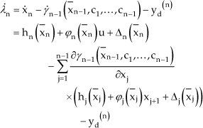
When i = n – 1, (17) can be rewritten as:

{\dot{V}}_{n - 1} \leq - \sum_{j = 1}^{n - 1} c_{i} λ_{i}^{2} + φ_{n - 1} ({\bar{x}}_{n - 1}) λ_{n - 1} λ_{n}

(18)

Step n: In this step the practical control input u will be constructed to make $λ_{n} = x_{n} - γ_{n - 1} ({\bar{x}}_{n - 1}, c_{1}, \dots, c_{n - 1}) - y_{d}^{(n - 1)}$ as small as possible.

The time derivative of λ_n is given by:

\begin{array}{l} {\dot{λ}}_{n} = {\dot{x}}_{n} - {\dot{γ}}_{n - 1} ({\bar{x}}_{n - 1}, c_{1}, \dots, c_{n - 1}) - y_{d}^{(n)} \\ = h_{n} ({\bar{x}}_{n}) + φ_{n} ({\bar{x}}_{n}) u + Δ_{n} ({\bar{x}}_{n}) \\ - \sum_{j = 1}^{n - 1} \frac{\partial γ_{n - 1} ({\bar{x}}_{n - 1}, c_{1}, \dots, c_{n - 1})}{\partial x_{j}} \\ \times (h_{j} ({\bar{x}}_{j}) + φ_{j} ({\bar{x}}_{j}) x_{j + 1} + Δ_{j} ({\bar{x}}_{j})) \\ - y_{d}^{(n)} \end{array}

(19)

We choose c_n ∈ ℝ such that

c_{n} > 0

(20)

We consider the Lyapunov function candidate:

V_{n} = V_{n - 1} + \frac{1}{2} λ_{n}^{2}

(21)

The time derivative of V_n is

\begin{array}{l} {\dot{V}}_{n} = {\dot{V}}_{n - 1} + {\dot{λ}}_{n} λ_{n} \\ \leq - \sum_{j = 1}^{n - 1} c_{i} λ_{i}^{2} + h_{n} ({\bar{x}}_{n}) λ_{n} \\ + l_{n} \tanh (ρ λ_{n}) λ_{n} \\ + φ_{n} ({\bar{x}}_{n}) u λ_{n} - y_{d}^{(n)} λ_{n} \\ + φ_{n - 1} ({\bar{x}}_{n - 1}) λ_{n - 1} λ_{n} \\ - \sum_{j = 1}^{n - 1} \frac{\partial γ_{n - 1} ({\bar{x}}_{n - 1}, c_{1}, \dots, c_{n - 1})}{\partial x_{j}} λ_{n} \\ \times (h_{j} ({\bar{x}}_{j}) + φ_{j} ({\bar{x}}_{j}) x_{j + 1} \\ - l_{j} \tanh (ρ λ_{n} \frac{\partial γ_{n - 1} ({\bar{x}}_{n - 1}, c_{1}, \dots, c_{n - 1})}{\partial x_{j}})) \end{array}

(22)

At the end of the backstepping procedure, we take:

\begin{array}{l} u = \frac{1}{φ_{n} ({\bar{x}}_{n})} (\sum_{j = 1}^{n - 1} \frac{\partial γ_{n - 1} ({\bar{x}}_{n - 1}, c_{1}, \dots, c_{n - 1})}{\partial x_{j}} \\ \times (h_{j} ({\bar{x}}_{j}) + φ_{j} ({\bar{x}}_{j}) x_{j + 1} \\ - l_{j} \tanh (ρ λ_{n} \frac{\partial γ_{n - 1} ({\bar{x}}_{n - 1}, c_{1}, \dots, c_{n - 1})}{\partial x_{j}})) \\ - c_{n} λ_{n} - h_{n} ({\bar{x}}_{n}) \\ - l_{n} \tanh (ρ λ_{n}) + y_{d}^{(n)} - φ_{n - 1} ({\bar{x}}_{n - 1}) λ_{n - 1}) \end{array}

(23)

Then, the time-derivative of V_n satisfies the following condition:

{\dot{V}}_{n} \leq - \sum_{j = 1}^{n} c_{i} λ_{i}^{2}

(24)

Let us consider:

{\begin{matrix} c_{i} \geq \frac{μ}{2} > 0 \\ \forall i = 1, \dots, n \end{matrix}

(25)

Therefore, we obtain:

{\dot{V}}_{n} \leq - μ V_{n} \leq 0

(26)

Theorem 1. Suppose that the proposed control method in this section is applied to the system (1). Then, for any initial conditions, the closed-loop system is globally stable for t ∈ [0,∞[. Moreover, the tracking error converges to zero, i.e., e(t)→ 0 as t → ∞.

Proof. By means of the Barbalat lemma [17, 18], we have

\lim_{t \to \infty} V_{n} (t) = 0

(27)

This implies that:

\lim_{t \to \infty} λ_{1} (t) = 0

(28)

From (28), it is easy to see that

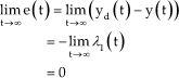
\begin{array}{l} \lim_{t \to \infty} e (t) = \lim_{t \to \infty} (y_{d} (t) - y (t)) \\ = - \lim_{t \to \infty} λ_{1} (t) \\ = 0 \end{array}

(29)

This completes the proof.

4. Simulation examples and discussion

In this section, the feasibility of the proposed method and the control performances are illustrated with three examples. The simulation results are carried out using the software MATLAB.

Example 1

For the simulation example 1, we consider the following nonlinear system

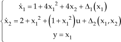
{\begin{matrix} {\dot{x}}_{1} = 1 + 4 x_{1}^{2} + 4 x_{2} + Δ_{1} (x_{1}) \\ {\dot{x}}_{2} = 2 + x_{1}^{2} + (1 + x_{1}^{2}) u + Δ_{2} (x_{1}, x_{2}) \\ y = x_{1} \end{matrix}

(30)

where: u and y are the control signal and measured output, respectively; |Δ₁(x₁)|≤0.1 and|Δ₂(x₁, x₂)| ≤ 0.2. The aim of the control is to force the output y = x₁ to asymptotically track a reference signal y_d. Using the controller design procedure described in section 3, we can write:

\begin{array}{l} n = 2, h_{1} (x_{1}) = 1 + 4 x_{1}^{2}, h_{2} (x_{1}, x_{2}) = 2 + x_{1}^{2}, φ_{1} (x_{1}) = 4, \\ φ_{2} (x_{1}, x_{2}) = 1 + x_{1}^{2}, λ_{1} = x_{1} - y_{d}, l_{1} = 0.1, l_{2} = 0.2, \\ γ_{1} (x_{1}, c_{1}) = \frac{1}{4} (c_{1} y_{d} - c_{1} x_{1} - 1 - 4 x_{1}^{2} - 3 {\dot{y}}_{d} - 0.1 \tanh (ρ x_{1} - ρ y_{d})), \\ λ_{2} = x_{2} - \frac{1}{4} (c_{1} y_{d} - c_{1} x_{1} - 1 - 4 x_{1}^{2} + {\dot{y}}_{d} - 0.1 \tanh (ρ x_{1} - ρ y_{d})) . \end{array}

We choose c₁ = 1, c₂ = 2 and ρ = 10⁵.

Then, the control input becomes:

\begin{array}{l} u = \frac{1}{1 + x_{1}^{2}} (\frac{\partial γ_{1} (x_{1}, c_{1})}{\partial x_{1}} (1 + 4 x_{1}^{2} + 4 x_{2} \\ - 0.1 \tanh (10^{5} λ_{2} \frac{\partial γ_{1} (x_{1}, c_{1})}{\partial x_{1}})) \\ - 2 λ_{2} - 2 - x_{1}^{2} \\ - 0.2 \tanh (10^{5} λ_{2}) + {\ddot{y}}_{d} - 4 x_{1} + 4 y_{d}) \end{array}

(31)

Such as

\frac{\partial γ_{1} (x_{1}, c_{1})}{\partial x_{1}} = - 0.25 - 2 x_{1} - 2500 + 2500 \tanh^{2} (10^{5} x_{1} - 10^{5} y_{d})

(32)

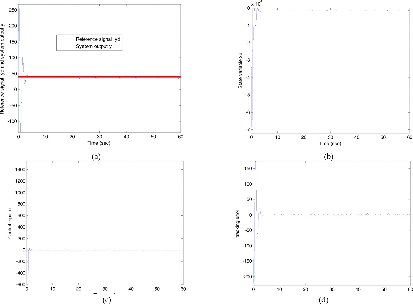
The simulation results for the initial states (x₁(0) = 20,x₂(0) = −25) are shown in figures 1-2. It can be seen that the output of the closed-loop system tracks the reference signals.

Figure 1.

Simulation results if y_d = 40: (a) system output y = x₁ and the reference signal y_d; (b) State variable x₂; (c) control input u; (d) tracking error y_d-y

Figure 2.

Simulation results if $y_{d} (t) = 40 sin (\frac{2 π}{10} t)$ : (a) system output y = x₁ and the reference signal y_d; (b) State variable x₂; (c) control input u; (d) tracking error y_d – y

Example 2

For the simulation example 2, we consider the nonlinear system, which is described as

{\begin{matrix} {\dot{x}}_{1} = \sqrt{1 + 6 x_{1}^{2}} + 5 x_{2} + Δ_{1} (x_{1}) \\ {\dot{x}}_{2} = 2 + \sqrt{x_{1}^{2} + 3 x_{2}^{2}} + (1 + x_{1}^{2} + 3 x_{2}^{2}) u + Δ_{2} (x_{1}, x_{2}) \\ y = x_{1} \end{matrix}

(33)

where: u and y are the control signal and measured output, respectively; |Δ₁ (x₁)| ≥ 10 and |Δ₂ (x₁,x₂)| ≥ 20.

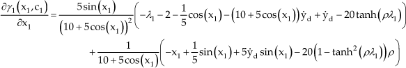
The objective of the control is to force the output y = x₁ to asymptotically track a reference signal y_d. According to the described controller design procedure in section 3, we have:

\begin{matrix} n = 2, h_{1} (x_{1}) = \sqrt{1 + 6 x_{1}^{2}}, h_{2} (x_{1}, x_{2}) = 2 + \sqrt{x_{1}^{2} + 3 x_{2}^{2}}, \\ φ_{1} (x_{1}) = 5, φ_{2} (x_{1}, x_{2}) = 1 + x_{1}^{2} + 3 x_{2}^{2}, l_{1} = 10, l_{2} = 20, \\ λ_{1} = x_{1} - y_{d}, \\ γ_{1} (x_{1}, c_{1}) = \frac{1}{5} (c_{1} y_{d} - c_{1} x_{1} - \sqrt{1 + 6 x_{1}^{2}} - 4 {\dot{y}}_{d} - 10 \tanh (ρ x_{1} - ρ {\dot{y}}_{d})), \\ λ_{2} = x_{2} - \frac{1}{5} (c_{1} y_{d} - c_{1} x_{1} - \sqrt{1 + 6 x_{1}^{2}} - {\dot{y}}_{d} - 10 \tanh (ρ x_{1} - ρ {\dot{y}}_{d})) . \end{matrix}

We choose c₁ = 1 and c₂ = 2.

Then, we can obtain the control input

\begin{array}{l} u = \frac{1}{1 + x_{1}^{2} + 3 x_{2}^{2}} (\frac{\partial γ_{1} (x_{1}, c_{1})}{\partial x_{1}} (\sqrt{1 + 6 x_{1}^{2}} + 5 x_{2} \\ - 10 \tanh (ρ λ_{2} \frac{\partial γ_{1} (x_{1}, c_{1})}{\partial x_{1}})) \\ - 2 λ_{2} - 2 - \sqrt{x_{1}^{2} + 3 x_{2}^{2}} \\ - 20 \tanh (ρ λ_{2}) + {\ddot{y}}_{d} - 5 x_{1} + 5 y_{d}) \end{array}

(34)

Such that

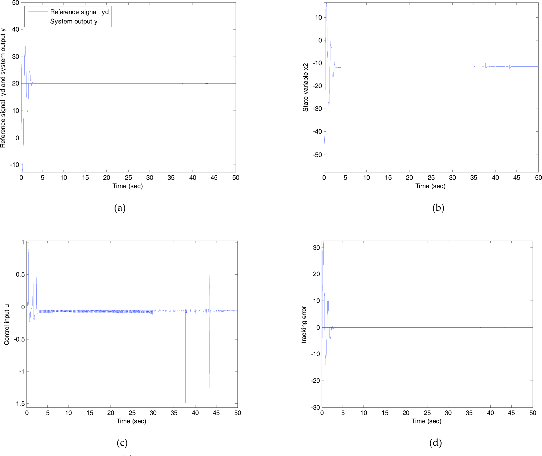
\frac{\partial γ_{1} (x_{1}, c_{1})}{\partial x_{1}} = \frac{1}{5} (- 1 - \frac{12 x_{1}}{\sqrt{1 + 6 x_{1}^{2}}} - 10 ρ + 10 ρ \tanh^{2} (ρ x_{1} - ρ y_{d}))

(35)

For the initial states (x₁ (0) = 50, x₂ (0) = −50), simulation results are presented in figures 3 -6. From the results, we find that the output of the closed-loop system tracks the reference signals. It can be seen that the chattering amplitudes have been effectively reduced where ρ = 100 compared to where ρ = 10⁵.

Figure 3.

Simulation results if $y_{d} (t) = 10 sin (\frac{2 π}{20} t)$ and $ρ = 10^{5}$ : (a) system output y = x₁ and the reference signal y_d; (b) State variable x₂; (c) control input u; (d) tracking error y_d – y

Figure 4.

Simulation results if $y_{d} (t) = 10 sin (\frac{2 π}{20} t)$ and $ρ = 100$ : (a) system output y = x₁ and the reference signal y_d; (b) State variable x₂; (c) control input u; (d) tracking error y_d – y

Figure 5.

Simulation results if y_d (t) = 20 and ρ = 10⁵: (a) system output y = x₁ and the reference signal y_d; (b) State variable x₂; (c) control input u; (d) tracking error y_d – y

Figure 6.

Simulation results if y_d (t) = 20 and ρ = 100: (a) system output y = x₁ and the reference signal y_d; (b) State variable x₂; (c) control input u; (d) tracking error y_d – y

Example 3

For simulation example 3, we consider the following nonlinear system, which is defined as

{\begin{matrix} {\dot{x}}_{1} = 2 + \frac{1}{5} \cos (x_{1}) + (10 + 5 \cos (x_{1})) x_{2} + Δ_{1} (x_{1}) \\ {\dot{x}}_{2} = 1 + \cos^{2} (x_{1} + x_{2}) + (2 + \sin^{2} (x_{1})) u + Δ_{2} (x_{1}, x_{2}) \\ y = x_{1} \end{matrix}

(36)

where: u and y are the control signal and measured output, respectively; |Δ₁ (x₁)| ≤ 20 and |Δ₂ (x₁,x₂)| ≤ 30.

The objective of the control is to force the output y = x₁ to asymptotically track a reference signal yd. According to the described controller design procedure in section 3, we have:

\begin{array}{l} n = 2, h_{1} (x_{1}) = 2 + \frac{1}{5} \cos (x_{1}), \\ h_{2} (x_{1}, x_{2}) = 1 + \cos^{2} (x_{1} + x_{2}), φ_{1} (x_{1}) = 10 + 5 \cos (x_{1}), \\ φ_{2} (x_{1}, x_{2}) = 2 + \sin^{2} (x_{1}), l_{1} = 20, l_{2} = 30, λ_{1} = x_{1} - y_{d}, \\ γ_{1} (x_{1}, c_{1}) = \frac{1}{10 + 5 \cos (x_{1})} (- c_{1} λ_{1} - 2 - \frac{1}{5} \cos (x_{1}) \\ - (10 + 5 \cos (x_{1})) {\dot{y}}_{d} \\ + {\dot{y}}_{d} - 20 \tanh (ρ λ_{1})) \\ λ_{2} = x_{2} - \frac{1}{10 + 5 \cos (x_{1})} (- c_{1} λ_{1} - 2 - \frac{1}{5} \cos (x_{1}) + {\dot{y}}_{d} - 20 \tanh (ρ λ_{1})) . \end{array}

We choose c₁ = 1 and c₂ =2.

Then, the control input is designed as

\begin{array}{l} u = \frac{1}{2 + \sin^{2} (x_{1})} (\frac{\partial γ_{1} (x_{1}, c_{1})}{\partial x_{1}} (2 + \frac{1}{5} \cos (x_{1}) + (10 + 5 \cos (x_{1})) x_{2} \\ - 20 \tanh (ρ λ_{2} \frac{\partial γ_{1} (x_{1}, c_{1})}{\partial x_{1}})) \\ - 2 λ_{2} - 1 - \cos^{2} (x_{1} + x_{2}) \\ - 30 \tanh (ρ λ_{2}) + {\ddot{y}}_{d} - (10 + 5 \cos (x_{1})) λ_{1}) \end{array}

(37)

Such that

\begin{matrix} \frac{\partial γ_{1} (x_{1}, c_{1})}{\partial x_{1}} = \frac{5 \sin (x_{1})}{{(10 + 5 \cos (x_{1}))}^{2}} (- λ_{1} - 2 - \frac{1}{5} \cos (x_{1}) - (10 + 5 \cos (x_{1})) {\dot{y}}_{d} + {\dot{y}}_{d} - 20 \tanh (ρ λ_{1})) \\ + \frac{1}{10 + 5 \cos (x_{1})} (- x_{1} + \frac{1}{5} \sin (x_{1}) + 5 {\dot{y}}_{d} \sin (x_{1}) - 20 (1 - \tanh^{2} (ρ λ_{1})) ρ) \end{matrix}

(38)

Figure 7.

Simulation results if y_d (t) = 100 and ρ = 100: (a) system output y = x₁ and the reference signal y_d; (b) State variable x₂; (c) control input u; (d) tracking error y_d – y

For the initial states (x₁ (0) = 10,x₂ (0) = −10), the results of the simulation are shown in figures 7 -10. It can be concluded that the output of the closed-loop system tracks the reference signals very well. The value of the parameter ρ has an influence on the chattering amplitudes. Furthermore in the three examples, we notice that all the signals of the resulting closed-loop systems are regularly bounded and the tracking error converges to zero.

Figure 8.

Simulation results if y_d (t) = 100 and ρ = 10⁵: (a) system output y = x₁ and the reference signal y_d; (b) State variable x₂; (c) control input u; (d) tracking error y_d – y

Figure 9.

Simulation results if y_d(t) = sin(πt) and ρ = 100: (a) system output y = x₁ and the reference signal y_d; (b) State variable x₂; (c) control input u; (d) tracking error y_d – y

Figure 10.

Simulation results if y_d (t) = sin(πt) and ρ = 10⁵: (a) system output y = x₁ and the reference signal y_d; (b) State variable x₂; (c) control input u; (d) tracking error y_d – y

5. Conclusion

In this paper, we propose a method of designing an adaptive controller for a class of nonlinear systems using the backstepping technique. The on-line calculation of the control input is obtained using the Lyapunov synthesis approach. The proposed approach guarantees that all the signals of the resulting closed-loop systems are regularly bounded and the tracking error converges to zero. It has advantages, such as a simple structure, easy realization, a good control effect and strong robustness. The efficiency of the proposed control has been demonstrated by simulation studies. Future works could expand the method to be used for a more general class of uncertain nonlinear systems.

References

Nguyen

N. T.

, “Optimal control modification for robust adaptive control with large adaptive gain,” Systems & Control Letters, vol. 61, No. 4, pp. 485–494, 2012.

Chen

Qin

Sun

Fang

, “Global adaptive neural network control for a class of uncertain non-linear systems,” IET Control Theory Applications, vol. 5, No. 5, pp. 655–662, 2011.

Montaseri

Yazdanpanah

M. Javad

, “Adaptive control of uncertain nonlinear systems using mixed backstepping and Lyapunov redesign techniques,” Communications in Nonlinear Science and Numerical Simulation, vol. 17, No. 8, pp. 3367–3380, 2012.

Hamida

M. Assaad

Glumineau

de Leon

, “Robust integral backstepping control for sensorless IPM synchronous motor controller,” Journal of the Franklin Institute, vol. 349, No. 5, pp. 1734–1757, 2012.

H.-Yan

Y.-An

Ren

Cun J.

Zhu

, “Dynamic Feedback Backstepping Control for a Class of MIMO Nonaffine Block Nonlinear Systems,” Mathematical Problems in Engineering, vol. 2012(2012), Article ID 493715, 18 pages.

Zhu

Ling

Xie

, “Robust Adaptive Switching Control for Markovian Jump Nonlinear Systems via Backstepping Technique,” Journal of Applied Mathematics, vol. 2012(2012), Article ID 514504, 22 pages.

Mei

Jiang

, “Robust adaptive backstepping control for a class of uncertain nonlinear systems based on disturbance observers,” Science China Information Sciences, vol. 53, No. 6, pp. 1201–1215, 2010.

Dong

Farrell

J. A.

Polycarpou

M. M.

Djapic

Sharma

, “Command Filtered Adaptive Backstepping,” Control Systems Technology, IEEE Transactions on, vol. 20, No. 3, pp. 566–580, 2012.

Lin

F.-Jeng

Shieh

P.-Huang

Chou

P.-Huan

, “Robust Adaptive Backstepping Motion Control of Linear Ultrasonic Motors Using Fuzzy Neural Network,” Fuzzy Systems, IEEE Transactions on, vol. 16, No. 3, pp. 676–692, 2008.

10.

Chung

C.-Hsien

Chen

M.-Shin

, “A robust adaptive feedforward control in repetitive control design for linear systems,” Automatica, vol. 48, No. 1, pp. 183–190, 2012.

11.

Wang

Deng

Wei

Che

Wong

Y.K.

Chan

W.L.

Tsang

K.M.

, “Adaptive backstepping sliding mode control for chaos synchronization of two coupled neurons in the external electrical stimulation,” Communications in Nonlinear Science and Numerical Simulation, vol. 17, No. 3, pp. 1344–1354, 2012.

12.

Alfi

, “Chaos suppression on a class of uncertain nonlinear chaotic systems using an optimal H_∞ adaptive PID controller,” Chaos, Solitons & Fractals, vol. 45, No. 3, pp. 351–357, 2012.

13.

Zhang

, “Adaptive backstepping trajectory tracking control of robot manipulator,” Journal of the Franklin Institute, vol. 349, No. 3, pp. 1087–1105, 2012.

14.

Fang

Zhang

W. G. and L.

, “Robust adaptive integral backstepping control of a 3-DOF helicopter,” International Journal of Advanced Robotic Systems, vol. 9, Published 20 September, 2012.

15.

Mnif

, “Reccursive backstepping stabilization of a wheeled mobile robot,” International Journal of Advanced Robotic Systems, vol. 1, No. 4, pp. 287–294, 2004

16.

Dadras

Momeni

Reza H.

, “Adaptive sliding mode control of chaotic dynamical systems with application to synchronization,” Mathematics and Computers in Simulation, vol. 80, No. 12, pp. 2245–2257, 2010.

17.

, “Projective lag synchronization of the general complex dynamical networks with distinct nodes,” Communications in Nonlinear Science and Numerical Simulation, vol. 17, No. 11, pp. 4417–4429, 2012.

18.

Liu

, “Robust Adaptive Coordinated Attitude Control Problem with Unknown Communication Delays and Uncertainties,” Procedia Engineering vol. 29, pp. 1447–1455, 2012.