The Design and Cost Analysis of DCP Algorithm based on Directional Circle

Abstract

This paper proposed a theoretical analysis model of the DCP cost and its assumption. Repatrolling the regular network topologies of Grid and Hexagonal, it reasoned the relationship of DCP cost, the DCP parameter (start TTL a, the fixed increment value b, and the patrol threshold L), network size, and the node density out. In order to validate the conclusion, this paper simulated it with a lot of AODV-DCP experiments in the JiST/SWANS simulation platform. It provides a necessary theoretical basis for setting the DCP parameter.

1. Introduction

Almost all existing security risk patrols start by sending RSREQ in the network. This is widely used in the fixed network, but in the high speed moving network, this frequent patrol will exhaust the energy of every node rapidly and occupy the most available network bandwidth [1, 2].A possible solution: by setting a big enough value for TTL of RSREQ, make RSREQ both send to the destination node, and avoid over the full network [3]–[5]. However, the nodes do not know the global situation of network, so it is very difficult to determine the optimal TTL.

Patent [6] analyze the influence of the threshold of directional circle patrol on the cost of broadcast based on simulated annealing algorithm by establishing three different network topology – Ring, grid, six edge, and take experimental analysis in random network topology, and give a conclusion: There is a optimal threshold L, and its value is between 1 and 4. For the regular topology of network, although select carefully the directional limit, but it is insignificant to the reduction of broadcast cost. However, DCP is quite effective in reducing the cost of broadcast for the random network topology. But, patent [6] only study the performance of DCP in the case of that the initial value and directed fixed increment value of TTL are both 1.

Patent [7] by the experiments of establishing the theoretical model and random network topology (parameters: network size, hop), search for the existence of optimal directional threshold, and realize distributed multiple security authentication of the moving node, and can reduce the broadcast cost of DCP. The conclusion is: For any of the topology, the broadcast cost can be reduced by 12%–52% when directional threshold set for the best value. In the mathematical model, assume that the distribution of the required information in the network is equal probability, and the initial value and fixed increment value of DCP are both 1. At the same time, it proved the conclusions of the patent [6] once again. And get a conclusion that by increasing the initial value and fixed increment value can reduce the consumption of bandwidth and lock time.

Based on the above research achievements, this paper take high speed moving network in Strategic Internet environment as background, analysis the performance of DCP with different TTL initial value and directed fixed increment value, and provide a necessary theoretical basis for setting DCP parameters (The initial directional scope, fixed increment value and directional limit).

2. Modeling and derivation

As shown in figure 1, this paper establishes a general regular network topology to research this question. In this structure, we assume that every node can receive and send message by omnibearing Radio antenna. If node i within the radio range of node j, then node i and node j is neighbor (only one jump between them). The node that begins broadcast RSREQ is called host node. Each node has d nodes that distribute equably around it with equal distance, the host node is located in the center of the network, the rest of the nodes distribute equably in the network topology; we use char V to represent the number of hops between a node to patrol center, then one hop nodes in circle 1, two hop nodes in circle 2…r hop nodes in circle r (0<r<M, the network size is M hops). So, there are *** d × r nodes in circle r. Assume that host node is located in circle 0. We use f(r) to represent distribution function of nodes in every circle.

Figure 1.

structural model

$f(r)\{\begin{array}{ll}d\times r\hfill & r>0anddis\text{consta}\hfill \\ 1\hfill & r=0\hfill \end{array}$

(1)

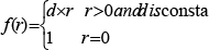
Visibly, the distribution function increase linearly in every circle.

The cost of retransmitting nodes' patrol information includes many aspects, such as processing cycle, the network bandwidth and so on. For analysis conveniently, in this paper, the unit of cost is the total number of nodes that retransmit RSREQ.

The model above is based on the fact: in Ad Hoc network, when a patrol message arrive a node that is i hops from sender, the patrol message must will be retransmitted by nodes which are located from 1 hop to i-1 hop. It is impossible that the message arrive receiver which is n (n>1) hops from the sender and there are no other nodes between sender and receiver. These characteristics also apply to other more jump network such as P2P network. In this paper, DCP is based on AODV, Because of the mechanism that restrains sending the copy of RSREQ in AODV, every node's location is fixed during a broadcast process.

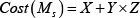
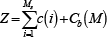
We use c(i) to represent the cost of patrolling circle i. In order to patrol nodes in circle i, all nodes in circle 1 - circle (i-1) will retransmit RSREQ message. Therefore, the total number of retransmission of RSREQ message equals the total number of messages being retransmitted in this circle and the first message sending by host node. In this way, we have

$c(i)=1+\sum _{k=1}^{i-1}{n}_k$

N_k is the total number of nodes in circle k. Assume that the probability we find RSREQ message in any node is equal when the host node sends RSREQ, so the probability of finding the message we need in circle i is :

$P\left(i\right)=\raisebox{1ex}{$n_i$}\!\left/ \!\raisebox{-1ex}{$\sum _{k=1}^M{n}_k$}\right.$

2.1 The directional function of patrol

When the current patrol failed, the directional function of patrol decides the growth way of TTL and makes a new TTL for the next patrol.

According to the present research and using of DCP, the growth ways of TTL are almost increasing linearly based on a fixed value such as 1 or 2. We use a to represent the initial value of TTL and b to represent the fixed increment value. If x represents the number of DCP patrol times, then the directional function of patrol f_e (x) can be defined as:

$f_e(x)=a+(x-1)b$

(2)

f_e(x) represents the TTL value when doing x time patrol, ms is integer and represent maximum number of patrol times. Because the maximum network size is M, we have f_e(ms)<M, it is a+(ms-1)b<M =>ms<(M-a)/b+1

2.2 The theoretical cost

Based on above model, the theoretical cost of DCP is made up of two major: (l)the cost of finding the target by patrol step by step when the information we need is located in the scope of patrol;(2) the cost of broadcasting through the full network when we cannot find the information we need. Patrol threshold L, i.e. the maximum value of TTL, the relationship between L and Ms is given as following:

$\begin{array}{l}f(x)<L\Rightarrow x\frac{L-a}{b}+1\Rightarrow Ms\le \frac{L-a}{b}+1\hfill \\ \Rightarrow Ms=\left[\frac{L-a}{b}+1\right]\hfill \end{array}$

(3)

DCP starts patrol with initial TTL = a, if failed, add b to the value of TTL. Therefore, the first time Ms=1 and TTL=a, if failed, the second time Ms=2 and TTL=a+b…until TTL=L.

Thus, the probability of finding the target in round x and the cost of DCP patrol in round x are :

$p(x)=\{\begin{array}{ll}\frac{{\sum }_{i=1}^a{n}_i}{{\sum }_{k=1}^M{n}_k}\hfill & x=1\hfill \\ \frac{{\sum }_{a+(x-2)b+1}^{a+(x-1)b}{n}_i}{{\sum }_{k=1}^M{n}_k}\hfill & 2\le x\le \frac{L-a}{b}+1\hfill \end{array}$

(4)

$c(x)=1+{\sum }_{i=1}^{a+(x-1)b-1}{n}_i$

(5)

n_i is the number of nodes in circle i. So the cost of broadcast through the full network is :

$c_b(M)=1+\sum _{i=1}^{m-1}{n}_i$

(6)

Using formula (1) to substitute in formula (4),(5), we get formula (7), (8):

$p(x)=\{\begin{array}{ll}\frac{a^2+a}{M^2+M}\hfill & x=1\hfill \\ \frac{2b^{2}x+2ab-3b^2+b}{M^2+M}\hfill & 2\le x\le \frac{L-a}{b}+1\hfill \end{array}$

(7)

$c(x)=1+d\frac{[a+(x-1)b][a+(x-1)b-1]}{2}$

(8)

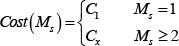
Cost (Ms) can be represented as the function of Ms, and formula (3) has given us the relationship between L and Ms.

$Cost(M_s)=X+Y\times Z$

(9)

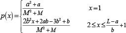
In formula (9), X generates by the part one of theory cost. This cost can be calculated by formula (10)

$X=\sum _{i=1}^{M_s}p(i)\times \sum _{k=1}^{i}c(k)$

(10)

For example, the patrol threshold L=2(directed initial value a=1 and directed fixed increment value b=1), we can conclude Ms=2 by formula (3). So,

$X=\sum _{i=1}^{2}p(i)\times \sum _{k=1}^{i}c(k)=p(1)+p(2)\times \left(c(1)+c(2)\right)$

Y × Z generates by the part two of theory cost. Y is the probability of finding target outside the patrol threshold and Z is the cost of patrol outside the patrol threshold. Y, Z can be calculated by formula (11), (12)

$Y=1-\sum _{i=1}^{M_s}p(i)$

(11)

$Z=\sum _{i=1}^{M_s}c(i)+C_{b}M$

(12)

Using Ms=0 to substitute in formula (9), Cost(0)≈C_b(M), therefore, Cost(Ms=0) means the cost of broadcast through full network without using DCP algorithm. After calculate, the cost function of DCP is

$Cost(M_s)=\{\begin{array}{ll}{C}_1\hfill & M_s=1\hfill \\ C_x\hfill & M_s\ge 2\hfill \end{array}$

(13)

In formula (13):

$\begin{array}{l}{C}_1=\frac{d{M}^4+(4-d-2ad)M^2+(2a^{2}d+4)M-2a^2-2a}{2(M^2+M)}\hfill \\ C_x=\frac{1}{60(M^2+M)}(-6d{b}^4{M}_s^5+30d{b}^3(b-a)M_s^4+10b^2(d(M^2+M+1+\hfill \\ 12ab-6a^2-5b^2-b)-2)M_s^3+15b(((2a-3b-1)M^2+(2a+b-1)M+\hfill \\ 2a-10a{b}^2-4a^3+12a^{2}b-2b-2ab+2b^2+2b^3)d+2b-4a-2)M_s^2+\hfill \\ (\left(\left(30a^2+65b^2-90ab-30a-15b\right)d+60\right)M^2+((30a^2-55b^2+30ab-\hfill \\ -30a+45b)d+60)M+(-60ab+60a{b}^2-15a^2{b}^2-30a^{2}b+60a{b}^3-20b^3\hfill \\ +20b^2+30a^2-30a^4+120a^{3}b-4b^4)d+30b-60a+60ab-60a^2-10b^2)M_s\hfill \\ +30d{M}^4+30\left(\left(2ab-a-b^2-a^2+b-1\right)d+2\right)M^2+30((-2ab+a^2+a\hfill \\ +b^2-b)d+2)M+30ab\left(1+ab-b-2a^2+a\right)d)\hfill \end{array}$

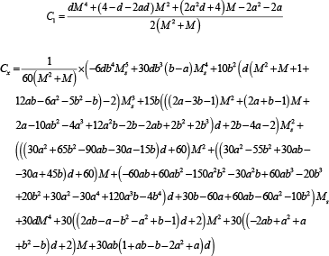
We can verify that C₁ = C_x [M_s = 1), therefore, Cost (M_s) = C_x

3. Cost analysis

In this section, we do further research with two typical topology structures: Grid and Hexagonal, as shown in figure 2. Grid model, each node has four neighbors node, i. e. d=4. Hexagonal model, d=6. Using d=4, 6 to substitute in formula (13), we get the model's theory cost formula.

Figure 2.

model topologies of Grid and Hexagonal

For example, if d=4,6 and a=1,b=1(in this situation, Ms=L), we get the theoretical cost expression of Grid and Hexagonal:

$\begin{array}{l}{C}_{gride}(L)=\frac{1}{15\left(M^2+M\right)}[-6L^5+\left(10M^2+10M+5\right)L^3+\left(-30M^2+30M-15\right)L^2+\hfill \\ \left(-25M^2+35M-14\right)L+30M^4-15M^2+15M]\hfill \\ C_{hex}(L)=\frac{1}{15\left(M^2+M\right)}[-9L^5+\left(15M^2+15M+10\right)L^3+\left(-45M^2+45M-15\right)L^2\hfill \\ +\left(-45M^2+45M-16\right)L+45M^2-30M^2+15M]\hfill \end{array}$

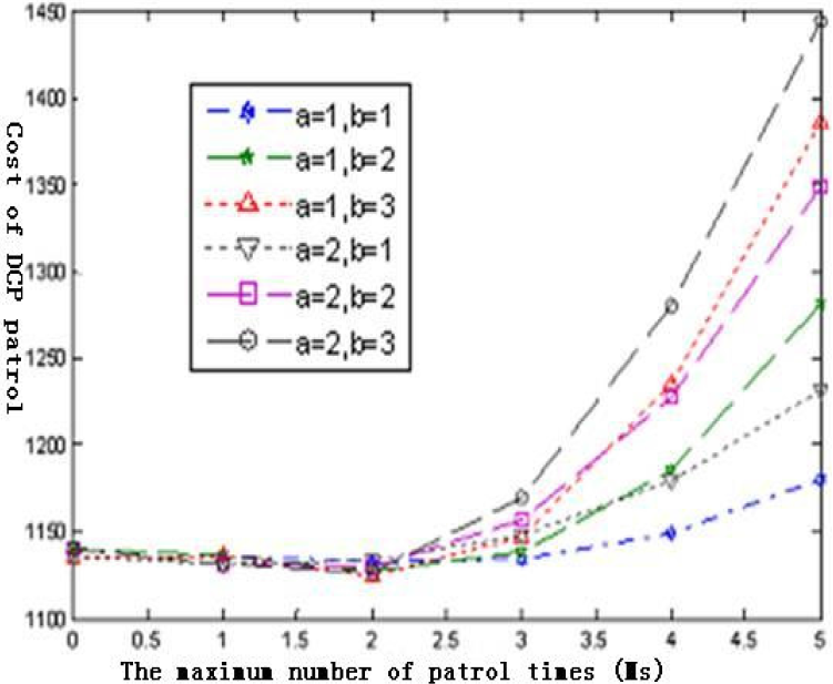
We analyze the performance of DCP algorithm by setting different parameter. We choice two typical network size (M=20, 50), the other network size have similar characteristic. In different network size, we analyze different cost curve of DCP by changing the initial value and fixed increment value of TTL. As shown in figure 3–figure 8. The X-coordinate denotes the maximum number of patrol times; Y-coordinate denotes the theory cost of DCP patrol. We can see from these figures: first, for all cost curves, we find DCP algorithm can reduce the cost of network broadcast by setting suitable parameter. However, along with the increase of number of patrol times, the cost will exceed pure broadcast without using DCP algorithm. From these cost curves, we can see that with the increase of the number of patrol times, the theoretical cost of DCP lower first, and then began to rise and more than the cost of full network broadcast.

Figure 3.

the cost curve of DCP in Grid when d=4,m=20

Figure 4.

the cost curve of DCP in Grid when d=4,m=50

Figure 5.

the cost curve of DCP in Hexagonal when d=6,m=20

Figure 6.

the cost curve of DCP in Hexagonal when d=6,m=50

Figure 7.

the cost curve of DCP when the density coefficient is 10 and m=20

Figure 8.

the cost curve of DCP when the density coefficient is 10 and m=50

As figure 3–figure 8, when patrol times less or equal to 2, no matter what type of network topology(d=4,6), no matter what the network size (M=20,50), no matter what the initial value of TTL (a=1,2), and no matter what fixed increment value(b=1,2,3), cost curves basically are overlapped. Specially, the theory cost is minimum when Ms=2. That is to say that the best number of patrol times (Ms) is 2 for the regular network.

If we exclude the difference on the numerical mark, we can think figure 3–figure 8 is the same. For example: when Ms is less than or equal to 2, the curves of different initial value and fixed increment value basically are overlapped. But when Ms is equal or greater than 2, the cost of patrol is more than the cost generating by pure full network broadcast (Ms = 0); when Ms is equal or greater than 4, the cost curve (A = 2, b = 2) exceed the cost curve(a = 2, b = 1), curve (a=1,b=3)and curve (a=2,b=2) have similar situation, This indicates that bigger fixed increment value have certain advantages if patrol times less than 4. But if patrol times more than 4, it is unwise to set big fixed increment value; if the initial TTL a is same, such as a=1, then with the increase of fixed increment value, the cost of patrol will increase in the same round.

In the model that density coefficient is 10:

As shown in formula (3), the relationship among Ms, the initial value a, the fixed increment value b and patrol threshold L is L = a + (M_s −1)b

Based on this above analysis, the best number of patrol times is Ms=2, we take the saving cost to measure the performance of DCP algorithm).

$\begin{array}{l}the\hspace{0.17em}\text{percentage of saving cost}=\hfill \\ \frac{\text{Cost}(0)-\text{Cost}(2)}{\text{Cost}(0)}\times 100\%\hfill \end{array}$

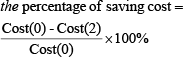
After calculate, we find that the saving cost of figure 3 and figure 6 are between 0.5% and 1.5%, the figure 4 and figure 7 are between 0.1% and 0.3%, and the figure 5 and figure 8 are about between 0.03% and 0.07%.

Visibly, No matter which type of network topology, along with the increase of the network size, the savings cost will drop.

4. The simulation

This paper simulated it with a lot of AODV-DCP experiments in the JiST/SWANS simulation platform. In order to compare and analyze conveniently, we test the influence of different parameter (Grid model and Hexagonal mode, the network size M=10, 20, initial value a=1, 2, 3 and fixed increment value b=1, 2) on the performance of DCP. We just change one parameter in one test. In different patrol threshold (maximum number of patrol times) Ms=1,2,3,4,5, we experiment many times to collect date, respectively. Because the target node is generated randomly, in order to make as far as possible each node at least have a chance to be the target node, we should ensure that the number of samples close to the number of nodes in network. When set the experiment parameter, Ms should be mapped to the patrol threshold T, the mapping formula is given in formula (3).

The methods of analyzing simulation data analysis accord to the thought of the theoretical derivation.

The results of processing simulation data as shown in figure 9–12. Through observation, we can find that in any topological model and any parameter, the maximum number of patrol times Ms between 1 and 3 when the cost of DCP is minimum, and Ms = 2 is in the majority. This result is close to the theoretical analysis. We can find that when Ms = 1, 2, 3, the cost of DCP is very close, and it is also acceptable. Therefore, in order to achieve the best of savings cost, we can consider according to type (3), setting the number of directional patrol times for 2 when set DCP parameter. Of course, according to the actual load condition of network, set the number of patrol times for 1 or 3 is also feasible.

We can still find that there is an obvious difference between the cost of pure broadcast and theoretical cost. As shown in figure 9 and figure 10, Grid model, M = 10, theoretically the cost is 181, but the actual is only 135 or so, reduce 25.4%; M = 20, the cost should be 761 in theory, but the actual is only 595 or so, reduce 21.8%. As shown in figure 11 and figure 17, Hexagonal model, M = 10, theoretically the cost is 270, but the actual is only 150 or so, reduce 44.4%; M = 20, the cost should be 1140 in theory, but the actual is only 690 or so, reduced about 39.5%. This, to a certain extent, indicate that the influence of node density on the cost of patrol, density coefficient increases, the probability of the collision between nodes increases, the cost of patrol will drop, but this is not necessarily a good thing.

Figure 9.

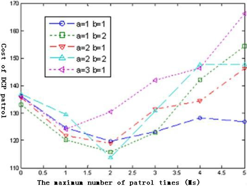
the simulation cost curve of DCP in Grid when m=10

Figure 10.

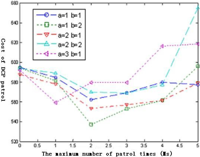
the simulation cost curve of DCP in Grid when m=20

Figure 11.

the simulation cost curve of DCP in Hexagonal when m=10

After calculate, we find that the saving cost of figure 9 are between 8.61% and 16.99%, figure 10 are between 2.11% and 9.63%, figure 11 are about between 7.55% and 17.00%, and figure 12 are about between 3.15% and 6.39%. Visibly, in the same network model, if the network bigger, the saving of cost is more obvious.

Figure 12.

the simulation cost curve of DCP in Hexagonal when m=20

In the process of simulation, the simulation data is got when the initial routing tables of each node are empty and this result in that it can't reveal fully the function of AODV agreement. In the actual network, after a period of running, each node in the network more or less has the routing to other nodes. From the point of view of statistics, host node and the neighbor node (including a few jumps within the scope of the node) have greater probability for exchanging information. Therefore, we can sure that the performance of DCP algorithm will embody more adequately, there is reason to believe that setting the number of patrol times for 2 is optimal.

This conclusion can also be used in security clustering algorithm of Ad Hoc network. In order to reduce the network load bringing by broadcast RSREQ information and increase network extensibility, we can schedule safety clustering algorithm, and send RSREQ to cluster head, checking routing information between clusters head when we can't find target node after two times patrol. Its function is similar to border router in the autonomous system in limited network.

5. Conclusion

This paper mainly studies the influence of different parameters on the performance of directional circle patrol (DCP) algorithm. We established the theoretical model and the hypothesis based on this model, and we calculate and analyze the theoretical cost of DCP in the model. Based on Grid and Hexagonal model, we study the relationship among the parameter (the initial value of TTL a, fixed increment value of TTL b, patrol threshold L), the network size, density coefficient of nodes and the cost of DCP. We find that the best number of patrol times is 2. And we prove this conclusion by a lot of experiments.