
Abstract
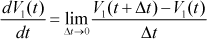
This article discusses the very crucial subject of RFID TAG's stability. RFID equivalent circuits of a label can be represented as Parallel circuits of Capacitance (Cpl), Resistance (Rpl), and Inductance (Lpc). We define V(t) as the voltage that develops on the RFID label therefore making dV(t)/dt the voltage-time derivative. Due to electromagnetic interference, there are different time delays with respect to RFID label voltages and voltage time derivatives. We define V1(t) as V(t) and V2(t) as dV(t)/dt. The delayed voltage and voltage derivative are V1(t-τ1) and V2(t-τ2) respectively (τ***1=τ2). The RFID equivalent circuit can be represented as a delayed differential equation that depends on variable parameters and delays. The investigation of RFID's differential equation is based on bifurcation theory [1], which is the study of possible changes in the structure of the orbits of a delayed differential equation as a function of variable parameters. This article first illustrates certain observations and analyzes local bifurcations of an appropriate arbitrary scalar delayed differential equation [2]. RFID label stability analysis is done under different time delays with respect to label voltage and voltage derivative. Additional analysis of the bifurcations of RFID's delayed differential equation on the circle. Bifurcation behavior of specific delayed differential equations can be condensed into bifurcation diagrams. This serves to optimize dimensional parameters analysis of RFID TAGs under electromagnetic interferences to get ideal performances.
1. Introduction
This article discusses a very critical and useful subject of passive RFID TAGs system stability analysis under electromagnetic interferences. RFID TAG system has two main variables—TAG-voltage and TAG-voltage derivative with respect to time which may be subject to delay as a result of electromagnetic interferences. We define τ1 as time delay respect to TAG's voltage and τ2 as time delay respect to TAG's voltage derivative. RFID Equivalent circuits of a Label can be represented as parallel circuits of Capacitance (Cpl), Resistance (Rpl), and Inductance (Lpc). Our RFID TAG system delay differential and delay differential model can be utilized for analysis of the dynamics of delay differential equations. Incorporation of a time delay is often necessary during some stage. It is often difficult to analytically study models with delay dependent parameters, even if only a single discrete delay is present. Practical guidelines exist that combine graphical information with analytical work to effectively study the local stability of models involving delay dependent parameters. The stability of a given steady state is determined simply through the use of the graphs of a function of τ1, τ2, which can be expressed distinctly and thus can be easily depicted by Matlab and other popular software–we need only look at one such function and locate the zeros. This function often has only two zeros, providing thresholds for stability switches. As time delay increases, the stability fluctuates. We emphasize the local stability aspects of certain models with delay-dependent parameters. In addition there is a general geometric criterion that, theoretically speaking may be applied to models that include many delays or even distributed delays. The simplest case is that of a first order characteristic equation which provides more user-friendly geometric and analytic criteria for stability switches. The analytical criteria provided for the first and second order cases can be used to obtain insightful analytical statements and can be helpful for conducting simulations.
2. RFID Equivalent Circuit and Representation of Delay Differential Equations
RFID TAG can be represented as a parallel Equivalent Circuit of Capacitor and Resistor in Parallel. For example, see NXP/PHILIPS ICODE IC Parallel equivalent circuit and simplified complete equivalent circuit of the label (L1 is the antenna inductance) [6].

NXP/PHILIPS ICODE IC Parallel equivalent circuit and simplified complete equivalent circuit of the label (L1 represents the antenna inductance).


RFID's coil dimensional parameters

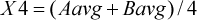
a0, b0 – Overall dimensions of the coil. Aavg Bavg – Average dimensions of the coil, t –Track thickness, w –Track width, g –Gap between tracks. Nc -Number of turns, d – Equivalent diameter of the track. Average coil area; -Ac=Aavg * Bavg. Integration of all of these parameters gives the equations for inductance calculation:


The RFID's coil calculation inductance is

Definition of limits, Estimations: Track thickness t, Al and Cu coils (t > 30um).
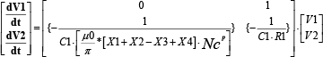
Due to electromagnetic interferences we get RFID TAG's voltage and voltage derivative with delays τ1 and τ2 respectively V1(t)→ V1(t- τ1); V2(t)→ V2(t- τ1). We consider no delay effect on dV1/dt and dV2/dt. The RFID TAG's differential equations under the effects of electromagnetic interferences (we consider electromagnetic interferences (delay terms) influence only RFID TAG voltage V1(t) and the voltage derivative V2(t) with respect to time. There is no influence on dV1(t)/dt and dV2(t)/dt):

To find the Equilibrium points (fixed points) of the RFID TAG system is by
We get two equations and the only fixed point is:

The RFID TAG system fixed values with arbitrarily small increments of exponential form [ν1 ν2]. eΛ·t are: i=0 (first fixed point), i=1 (second fixed point), i=2 (third fixed point).

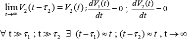
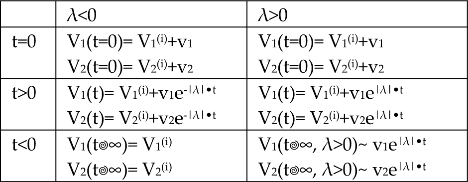
We choose the above expressions for our V1(t), V2(t) as small displacement [v1 v2] from the system's fixed points at time t=0.

When Λ < 0, t > 0 the selected fixed point is stable, however when Λ > 0, t > 0 is unstable. Our system tends towards the selected fixed point exponentially for Λ < 0, t > 0 and otherwise will deviate exponentially from the selected fixed point. Λ is the eigenvalue parameter which establishes whether the fixed point is stable or unstable. In addition, the absolute value (|Λ|) establishes the speed of flow toward or away from the selected fixed point [1] [2].
The speeds of flow toward or away from the selected fixed point for RFID TAG system voltage and voltage derivative respect to time are


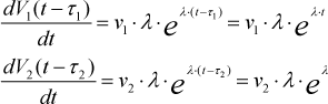
First we take the RFID TAG's voltage (Vi) differential equation:

Second we take the RFID TAG's voltage (V2) differential equation:


V1(i=0)=V2(i=0)=0 then v1/v2≈1;

If

then we have saddle fixed point otherwise it is an unstable node (both eigenvalues are positive). We define

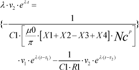
which gives us two delayed differential equations adding arbitrarily small increments of exponential form [ν1 ν2] · eΛ·t the coordinates [V1 V2].


In the equilibrium fixed point V1(i=0)=V2(i=0)=0 and

Then we get
We define

The small Jacobian increments of our RFID TAG system


We have three stability analysis cases: τ1 = τ τ2 = 0 or τ2 = τ; τ1 = 0 or τ1 = τ2 = τ otherwise τ1 ≠ τ2.
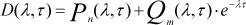
Just as in all of the above stability analysis cases, we need to identify characteristic equations. We study the occurrence of any possible stability switching resulting from the increase in value of the time delay τ for the general characteristic equation D(Λ, τ).
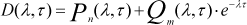
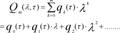
The expression for P n (Λ, τ) is

The expression for Q m (Λ, τ) is
3. RFID Tag System Second Order
CHARACTERISTIC EQUATION τ1 = τ τ2 = 0
The first case we analyze involves a delay in RFID Label voltage with no delay in voltage time derivative [4] [5].

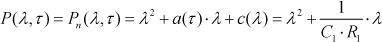
The expression for P n (Λ, τ) is

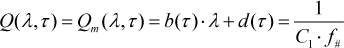
The expression for Q m (Λ, τ) is

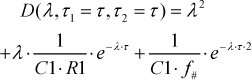
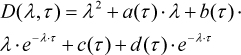
Our RFID system second order characteristic equation is:

Then

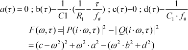
τ ε R+0 and a(τ), b(τ), c(τ), d(τ): R+0 → R are differentiable functions of class C1 (R+0) such that
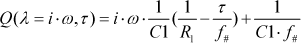
We assume that Pn (Λ, τ) = Pn (Λ) and Qm (Λ, τ) = Qm (Λ) cannot have common imaginary roots. That is, for any real number ω;


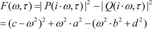
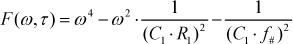
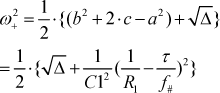
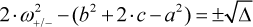
And its roots are given by


Therefore the following holds true:


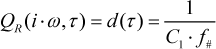
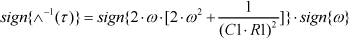
Q I (i · ω, τ) = ω(τ) · b = 0 hence


Which jointly with

defines the maps

which are continuous and differentiable in τ based on Lema 1.1 (see Appendix A). Hence we use theorem 1.2 (see Appendix B). This proves theorem 1.3 (see Appendix C) and theorem 1.4 (see Appendix D).
4. RFID Tag System Second Order
CHARACTERISTIC EQUATION τ1 =0; τ2 = τ
The second case we analyze involves no delay in RFID Label voltage but does have a delay in voltage time derivative [5].


The expression for P n (Λ, τ) is

The expression for Q m (Λ, τ) is

Our RFID system second order characteristic equation:

Then

And like in our previous case analysis:


we assume that Pn(Λ, τ) = P n (τ)and Qm(Λ, τ) = Qm(τ) cannot have common imaginary roots. That is, for any real number ω;


Therefore F(ω, τ) = 0 implies
And its roots are given by


Therefore the following holds:

Furthermore


Which, along with

Defines the maps
Defines the maps
which are continuous and differentiable in τ based on Lema 1.1 (see Appendix A). Hence we use theorem 1.2 (see Appendix B). This proves the theorem 1.3 (see Appendix C) and theorem 1.4 (see Appendix D).
5. RFID Tag System Second Order
CHARACTERISTIC EQUATION τ1 = τ; τ2 = τ
The third case we analyze is when there is delay in both the RFID Tabel voltage and in the voltage time derivative [4] [5].


The expression for P n (Λ, τ) is

The expression for Q m (Λ, τ) is

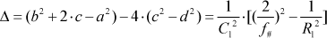
Taylor expansion:
since we need n > m for [BK] analysis we choose e−Λτ ≈ 1 – Λ · τ then we get


Our RFID system second order characteristic equation:
Then

And much like our previous case analysis:


we assume that P n (Λ, τ) = P n (Λ) and Q m (Λ, τ) can't have common imaginary roots. That is for any real number


Hence F(ω, τ) = 0 implies that:


The expressions for U and V can be derived easily [BK]:


Defines the maps Sn (τ) = τ – τ n (τ); τ ε I, n ε ℕ0
Defines the maps Sn (τ) = τ – τ n (τ); τ ε I, n ε ℕ0 which are continuous and differentiable in τ based on Lema 1.1 (see Appendix A). Hence we use theorem 1.2 (see Appendix B). This proves theorem 1.3 (see Appendix C) and theorem 1.4 (see Appendix D).
6. RFID Tag System Stability Analysis under Delayed Variables In Time
Our RFID homogeneous system for v1, v2 leads to a characteristic equation for the eigenvalue Λ having the form

We use different parameter terminology in this case:

Additionally Pn(λ,τ)→P(λ);Qn(λ,τ)→Q(λ)
then


n, m ε ℕ0, n > m and a j , c j : R+0 → R are continuous and differentiable function of τ such that a0 + c0 ≠ 0. In the following ____, “—” denotes complex and conjugate. P(Λ), Q(Λ)
Are analytic functions in Λ and differentiable in τ.
The coefficients:
{a j (C1, R1), c j (C1, antenna parametrs)} ε ℝ depend on RFID C1, R1 values and antenna parameters but not on τ.
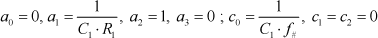
Unless absolutely necessary, the designation of the variation arguments (R1, C1, antenna parametrs) will subsequently be omitted from P, Q, aj, cj. The coefficients aj, cj are continuous, and differentiable functions of their arguments, and direct substitution shows that

∀ C1, antenna parameters ε ℝ+ i.e Λ = 0 is not a root of the characteristic equation. Furthermore P(Λ), Q(Λ) are analytic functions of Λ for which the following requirements of the analysis (see Kuang, 1993, section 3.4) can also be verified in the present case [4] [5].
If Λ = i · ω, ω ε ℝ then P(i · ω) + Q(i · ω) ≠ 0, i.e. P and Q have no common imaginary roots. This condition was verified numerically in the entire (R1, C1, antenna parametrs) domain of interest.
|Q(Λ) / P(Λ)| is bounded for | Λ | → ∞, Re Λ ≥ 0. No roots bifurcation from ∞.
Indeed, in the limit


Each positive root ω(C1, R1, antenna parametrs) of F(ω)=0 is continuous and differentiable with respect to C1, R1, antenna parametrs. This condition can only be assessed numerically.
In addition, since the coefficients in P and Q are real, we have
C1, R1, antenna parametrs and delay τ, ReΛ may, at the crossing, change its sign from (-) to (+), i.e. from a stable focus E(0)(V1(0), V2(0)) = (0, 0) to an unstable one, or vice versa.
This feature may be further assessed by examining the sign of the partial derivatives with respect to C1, R1 and antenna parameters.

antenna parameters = const; where ω ε ℝ+.
For the first case τ1 = τ; τ2 = 0 we get the following results


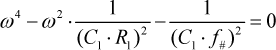
Q I (i · ω) = c1 · ω = 0; F(ω})=0 yield to


There are two options: first, it is always true that

Second

Not exist and always negative for any RFID TAG overall parameters values.
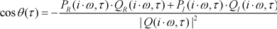
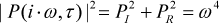
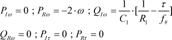
When writing P(Λ)=PR(Λ)+i·PI(Λ) and Q(Λ) = QR (Λ) + i · Q I (Λ), and inserting Λ = i · ω into RFID characteristic equation, ω must satisfy the following:


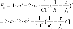
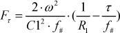
Where
Note that F(ω) is independent of τ. It is important to notice that if
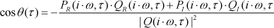
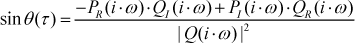
Then there are no positive ω(τ) solutions for F(ω, τ) = 0, and we cannot have stability switches. For any τ ε I where ω(τ) is a positive solution of F(ω, τ) = 0, we can define the angle θ(τ) ε [0,2 · π] as the solution of

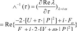
And ω(R1, C1, w,g,B0,A0,A AVG , BAVG etc.,), and keeping all parameters except one (x) and τ. The derivation closely follows that in reference [BK]. Differentiating RFID characteristic equation P(Λ) + Q(Λ) · e−Λ·τ =0 with respect to specific parameter (x), and inverting the derivative for convenience, one calculates:
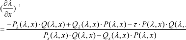

Upon separating this into real and imaginary parts, with


P2 = PR2+PI2. When (x) can be any RFID TAG parameters R1, C1, and time delay τ etc,. For convenience, we have dropped the arguments (i · ω, x), and


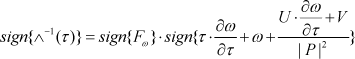
ω = −Fx/Fω. We define U and V:


We choose our specific parameter as time delay x = τ.


Differentiating with respect to τ, we get


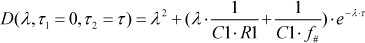
We now inspect the third interesting case wherein τ1 = τ; τ2 = τ when there are delays both in RFID Label voltage and voltage time derivative [4] [5].

Taylor expansion:

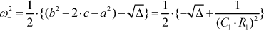
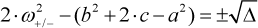
Hence F(ω, τ) = 0 implies

And its roots are given by


Therefore the following holds:


For our stability switching analysis we choose typical RFID parameter values: C1=23pF; R1=100kΩ=105; L calc =f#=2.65mH
Then
We find those ω, τ values which fulfill F(ω, τ) = 0. We ignore negative, complex, and imaginary values of ω for specific τ values. The following table gives the list. τ ε [0.001‥ 10] and can be expressed using a straight line(ω=τ·1.64·1013)
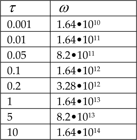

RFID TAG F(ω, τ) function for τ1=τ2=T
We plot the stability switch diagram based on different delay values of our RFID TAG system.


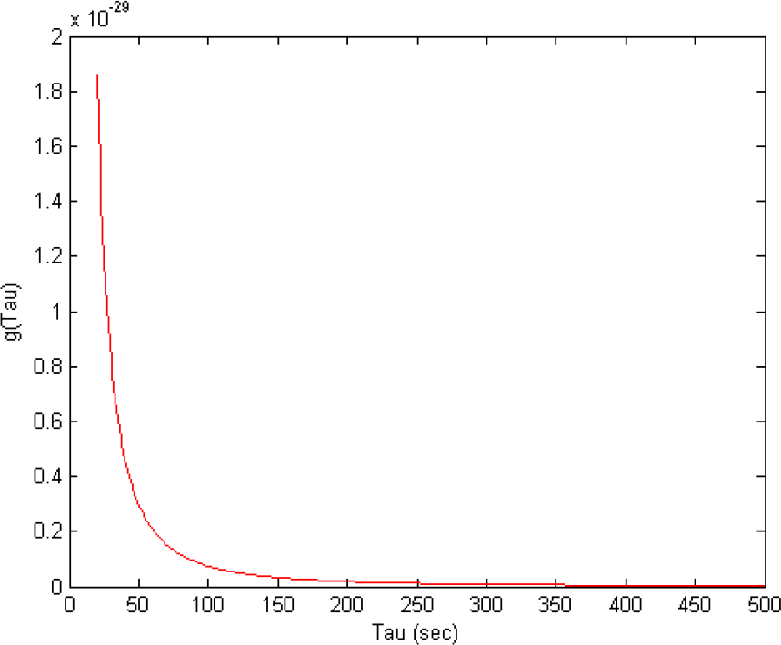
RFID TAG stability switch diagram based on different delay values of our RFID TAG system.
The stability switch occur only on those delay values (τ) that fit the equation:


When ω = ω+ (τ) if only ω+ is feasible. Additionally when all RFID TAG parameters are known, the stability switch due to various time delay values τ is described in the following expression:
7. Conclusion
A RFID TAG environment is characterize by electromagnetic interferences which can influence RFID TAGs stability in time. There are two main RFID TAGs variables which are affected by electromagnetic interferences– voltage developed on the RFID Label and the voltage time derivative. Each RFID Label variable under electromagnetic interference is characterized by respective time delay. The two time delays are not the same but can be categorized to some subcases due to interference behaviors.
The first case is when there is RFID Label voltage time delay but no voltage derivative time delay. The second case is when there is no RFID Label voltage time delay but there is a voltage derivative time delay. The third case is when both RFID Label voltage time delay and voltage derivative time delay exist. For simplicity we consider the two delays in the third case to be the same (the difference exists but it is negligible in our analysis). In each case we derive the related characteristic equation. The characteristic equation is dependent on the RFID Label's overall parameters and interference time delays. Following mathematical manipulation and [BK] theorems and definitions, we derived the expression which gives us a clear understanding of the RFID Label stability map. The stability map gives all possible options for stability segments where each segment belongs to different time delay values segments. RFID Label stability analysis can be influenced by TAG overall parameter values. We do not discuss this analysis in the current article.
Footnotes
Appendix A
Lemma 1.1
Assume that ω(τ)is a positive and real root of F(ω, τ) = 0
Defined for τ ε I, which is continuous and differentiable. Assume further that if Λ = i · ω, ω ε R, then P n (i · ω, τ) + Qn(i · ω, τ) ≠ 0, τ ε R hold true. Then the functions S n (τ) n ε N0, are continuous and differentiable on I.
Appendix B
Theorem 1.2
Assume that ω(τ)is a positive real root of F(ω, τ) = 0 defined for τ ε I, I ⊆ R+0, and at some τ* ε I, Sn(τ*) = 0
For some n ε N0 then a pair of simple conjugate pure imaginary roots Λ+(τ*)=i · ω(τ*), Λ_(τ*)= –i · ω(τ*) of D(Λ, τ) = 0 exist at τ = τ* which crosses the imaginary axis from left to right if δ(τ*) > 0 and crosses the imaginary axis from right to left if δ(τ*) < 0 where
The theorem becomes
Appendix C
Theorem 1.3
The characteristic equation: τ1 = τ, τ2 = 0; τ1 = 0, τ2 = τ
has a pair of simple and conjugate pure imaginary roots Λ = ±ω(τ*), ω(τ*)real at τ* ε I if S n (τ*)=τ*−τ n (τ*)=0 for some n ε N0. If ω(τ*) = ω+(τ*). This pair of simple conjugate pure imaginary roots crosses the imaginary axis from left to right if δ+(τ*) > 0 and crosses the imaginary axis from right to left if δ+ (τ*) < 0 where
If ω(τ*) = ω_ (τ*), this pair of simple conjugate pure imaginary roots cross the imaginary axis from left to right if δ_(τ*) > 0 and crosses the imaginary axis from right to left
If δ_(τ*) < 0 where
If ω+(τ*)=ω−(τ*)=ω(τ*) then Δ(τ*) = 0 and
The following result can be useful in identifying values of τ where there have been stability switches.
Appendix D
Theorem 1.4
Assume that for all τ ε I, ω(τ) is defined as a solution of F(ω, τ) = 0 then