Position/Force Control for a Single Leg of a Quadruped Robot in an Operation Space

Abstract

For a quadruped robot, to make full use of the sensors, especially the force sensor installed on the foot and adapt to the environment well, a kind of position/force control method is proposed in this paper. A quadruped mobile robot single leg model is established in this paper and its dynamic equation in a joint space is deduced by using the Lagrange equation. Then the model is transformed in the joint space into an operation space, based on the operation space coordinates, via kinematic relations. Next the new position/force control law on the base of the operation space dynamic equation is designed. In the end, the controller in the MatLab simulation environment is tested.

1. Introduction

Research on robots has lasted for decades. Many scholars have engaged in the work and achieved a lot of success. Most of the former studies were concentrated on kinematics and several representative biped robots came out, such as the Honda P series ^{[1, 2]}. In recent years, some scholars have used intelligent algorithms such as genetic algorithms ^[3], fuzzy algorithms ^[4] and optimizations ^[5] for walking planning and control. These methods indeed acquire some success in motion control, but they didn't deeply consider the reasons causing motions of robot. Controlling the leg position precisely is complicated for a highly nonlinear and strongly coupling quadruped mobile robot system. The problem is more difficult when considering environmental constraints on the feet. Constraints decrease the freedom dimensions and, because of mutual touch the leg bears a counterforce from the external environment, which will damage both the robot and the environment if it's too large, especially the counterforce in the vertical direction. The counterforce from the environment must be controlled effectively, in other words, the leg must be able to adapt to an unknown environment. Compliance control of the leg requires counterforce information, which can be achieved from the force sensor installed on the foot. However, it is difficult to use the force sensor in the joint space.

To overcome the problem of compliance and make full use of the force senor, we could consider solving the problem in the operation space. On the basis of such a thought, we design a position control law and a position/force control law in the horizontal direction and vertical direction respectively, where the position/force control law in vertical direction means dual loop control including outer position loop and inner force loop. The following sections will introduce the process of building a joint space model and an operation space model and how to design the controller.

2. Creating the Model

2.1 Joint Space Model

Figure 1 shows the structure of the single leg, which includes the body, thigh, calf and ankle. The single leg can be modelled as a four-link mechanical system, as shown in Figure 2(a). Every connecting rod rotates about the y axis in the x-z plane and point D touches the ground. In Figure 2(a) connecting rod 1 represents the body of the robot, whose centre of mass is at its geometrical centre, i.e., point A. Its mass and moment of inertia are, respectively, M_b and J_b. We don't care what attitude the body has, so we suppose the body moves in a horizontal direction. The second rod represents the thigh, whose centre of mass is the geometrical centre. Its mass, length and moment of inertia are, respectively, M₁, L₁ and. The angle θ_t = ∠A₁ AB and the driving torque between body and thigh is τ₁. The third rod represents the calf, whose centre of mass is the geometrical centre. Its mass, length and moment of inertia are, respectively, M₂, L₂ and J₂. The angle θ₂ = ∠ABC and the driving torque between thigh and calf is τ₂. The forth rod represents the ankle, whose centre of mass is also the geometrical centre. Its mass, length and moment of inertia are, respectively, M₃, L₃ and J₃. The angle θ₃ = ∠BCD and the driving torque between calf and ankle is τ₃.

Figure 1.

Single leg structure

Figure 2.

Simplified single leg model

Suppose there is a spring and damper installed on the foot, i.e., point D and the spring moves in a vertical direction. The length and rigidity coefficient of the spring are, respectively, r and K and the damping ratio is b, as shown in Figure 2(b).

Next we will deduce the joint space dynamic equation using the Lagrange method. A coordinate system on the robot is created and it is supposed that the coordinates of point A are (0, 0), so we can obtain the dynamic equation in the joint space as follows:

$\mathrm{A}(\theta )\ddot{\theta }+\mathrm{B}(\theta ,\dot{\theta })\dot{\theta }+\mathrm{G}(\theta )=\mathrm{C}\tau$

(1)

where θ = [θ₁;θ₂;θ₃;r], $\theta =\left[{\theta }_1;{\theta }_2;{\theta }_3;r\right]$ , $\ddot{\theta }$ is the joint angular acceleration and τ = [τ₁;τ₂;τ₃] is the joint driving torque. The controller design in the joint space is very mature, so Equation (1) is just the base of the operation space dynamic equation.

2.2 Operation Space Model

For a quadruped robot, our purpose is to control the position of body (point D), so we take X = [X_D;Z_D;r] as the generalized coordinates in the operation space. Because r is much smaller than the height of the leg, r can be overlooked when calculating Z_D.

The kinematic equation is as follows:

$\{\begin{array}{l}{\mathrm{X}}_{\mathrm{D}}={\mathrm{L}}_1\text{cos}{\theta }_1-{\mathrm{L}}_2\text{cos}({\theta }_2-{\theta }_1)+{\mathrm{L}}_3\text{cos}({\theta }_3-{\theta }_2+{\theta }_1)\\ {\mathrm{Z}}_{\mathrm{D}}=-({\mathrm{L}}_1\text{sin}{\theta }_1+{\mathrm{L}}_2\text{sin}({\theta }_2-{\theta }_1)+{\mathrm{L}}_3\text{sin}({\theta }_3-{\theta }_2+{\theta }_1))\\ \mathrm{r}=\mathrm{r}\end{array}$

(2)

According to kinematical transformation ^[6], the eliminating centrifugal force and the Coriolis force could achieve the dynamic equation in the operation space. The operation space dynamic equation is:

$\mathrm{M}(\mathrm{x})\ddot{\mathrm{X}}+\mathrm{G}(\mathrm{x})=\mathrm{F}$

(3)

Where:

$\begin{array}{l}\mathrm{M}(\mathrm{x})={\mathrm{J}}^{-\mathrm{T}}(\theta )\mathrm{A}(\theta ){\mathrm{J}}^{-1}(\theta )\\ \mathrm{G}(\mathrm{x})={\mathrm{J}}^{-\mathrm{T}}(\theta )\mathrm{G}(\theta )\\ \mathrm{F}={\mathrm{J}}^{-\mathrm{T}}(\theta )\mathrm{C}\tau \end{array}$

3. Controller Design

For a highly nonlinear and strongly coupling quadruped mobile robot system, designing the force control law for the single leg is complicated. In this paper we consider simplifying the single leg as a one-dimensional model at first, then progress to a multidimensional situation. The control block diagram of the single leg is shown in Figure 3.

Figure 3.

Control block diagram

3.1 One-dimensional Model

The one-dimensional model is shown in Figure 4, in which M is the mass of the body and the upper leg, m is the mass of the lower leg, F is the driving force and Z₁ and Z₂ are the height of the body and the lower leg. There is a spring and a damper between m and the ground, whose rigidity coefficient and damping ratio are, respectively, K and b. The force between the leg and ground is:

Figure 4.

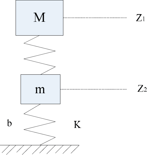
One-dimensional model

${\mathrm{F}}_{\mathrm{e}}=-\mathrm{K}{\mathrm{Z}}_2$

(4)

Suppose $x_1=Z_c=\frac{M{Z}_1+m{Z}_2}{M+m}$ , $x_2=-Z_2$ and take $x_1$ and $x_2$ as state variables.

When researching a manipulator arm, some scholars including Whitney ^[7], Salisbury ^[8], Hogan ^[9], Kazarooni ^[10], Maples and Becker ^[11], studied impedance control methods. On the basis of their work, a kind of position/force control law named Position Control Within Inner Force Loop (PCWIFL) is proposed in this paper. The control block diagram is shown in Figure 5.

Figure 5.

Control block diagram

In Figure 5:

${\mathrm{G}}_1(\mathrm{s})=\frac{{\mathrm{F}}_{\mathrm{e}}(\mathrm{s})}{{\mathrm{F}}_{\mathrm{d}}(\mathrm{s})}=\frac{\mathrm{K}}{\mathrm{m}{\mathrm{s}}^2+\mathrm{b}\mathrm{s}+\mathrm{K}}$

(5)

${\mathrm{G}}_2(\mathrm{s})=\frac{{\mathrm{Z}}_{\mathrm{c}}(\mathrm{s})}{{\mathrm{F}}_{\mathrm{e}}(\mathrm{s})}=\frac{\mathrm{b}\mathrm{s}+\mathrm{K}}{(\mathrm{m}+\mathrm{M}){\mathrm{s}}^2}$

(6)

Controller 1 is the position controller and Controller 2 is the inner loop force controller. Therefore, we have the following equation:

$\begin{array}{l}{\mathrm{F}}_{\mathrm{d}}=(\mathrm{M}+\mathrm{m})*\mathrm{g}+{\mathrm{k}}_{\mathrm{d}}({\dot{\mathrm{Z}}}_{\mathrm{c}\mathrm{d}}-{\dot{\mathrm{Z}}}_{\mathrm{c}})+{\mathrm{k}}_{\mathrm{p}}({\mathrm{Z}}_{\mathrm{c}\mathrm{d}}-{\mathrm{Z}}_{\mathrm{c}})\\ \mathrm{u}={\mathrm{F}}_{\mathrm{d}}+{\mathrm{k}}_{\mathrm{F}}({\mathrm{F}}_{\mathrm{d}}-{\mathrm{F}}_{\mathrm{e}})-\mathrm{m}\mathrm{g}\end{array}$

(7)

where k_d, k_p and k_F are the gain coefficients.

3.2 Multidimensional Single Leg

The model of a multidimensional single leg has been presented in Section 1. Considering that the body moves every time, the mass of the body must be taken into consideration. By rewriting Equation (3) we obtain the following dynamic equation:

$\left[\begin{array}{c}{{\mathrm{M}}^{\prime }}_{11}{{\mathrm{M}}^{\prime }}_{12}{{\mathrm{M}}^{\prime }}_{13}\\ {{\mathrm{M}}^{\prime }}_{21}{{\mathrm{M}}^{\prime }}_{22}{{\mathrm{M}}^{\prime }}_{23}\\ {{\mathrm{M}}^{\prime }}_{31}{{\mathrm{M}}^{\prime }}_{32}{{\mathrm{M}}^{\prime }}_{33}\end{array}\right]\left[\begin{array}{c}{\ddot{\mathrm{X}}}_{\mathrm{D}}\\ {\ddot{\mathrm{Z}}}_{\mathrm{D}}\\ \ddot{\mathrm{r}}+\mathrm{g}\end{array}\right]=\left[\begin{array}{c}{\mathrm{F}}_{\mathrm{X}}\\ {\mathrm{F}}_{\mathrm{Z}}\\ -\mathrm{b}\dot{\mathrm{r}}-\mathrm{K}\mathrm{r}\end{array}\right]$

(8)

in which:

$M^{\prime }=M+\left[\begin{array}{l}{M}_1\\ M_2\\ M_3\end{array}\right]=\left[\begin{array}{l}{M^{\prime }}_{11}{M^{\prime }}_{12}{M^{\prime }}_{13}\\ {M^{\prime }}_{21}{M^{\prime }}_{22}{M^{\prime }}_{23}\\ {M^{\prime }}_{31}{M^{\prime }}_{32}{M^{\prime }}_{33}\end{array}\right]$

and:

${\mathrm{M}}_1=\alpha {\mathrm{M}}_{\mathrm{b}},{\mathrm{M}}_2=\beta {\mathrm{M}}_{\mathrm{b}},{\mathrm{M}}_3={\mathrm{M}}_{\mathrm{b}},0<\alpha ,\beta <1$

Many scholars have done much research on force control of a mechanical arm in the operation space. Raibert and Craig proposed a kind of position/force control method ^[12]. Dr. Qing Wei discussed force control of mechanical arms in the operation space in detail in his doctoral dissertation ^[13]. We could design the controller in X and Z directions, respectively, based on different environmental constraints. In the horizontal direction, we adopt position control and the control law is as follows:

${\mathrm{F}}_{\mathrm{X}}={\mathrm{K}}_{\mathrm{p}\mathrm{x}}({\mathrm{X}}_{\mathrm{D}\mathrm{d}}-{\mathrm{X}}_{\mathrm{D}})+{\mathrm{K}}_{\mathrm{d}\mathrm{x}}({\dot{\mathrm{X}}}_{\mathrm{D}\mathrm{d}}-{\dot{\mathrm{X}}}_{\mathrm{D}})+{\ddot{\mathrm{X}}}_{\mathrm{D}\mathrm{d}}$

(9)

in which X_Dd is the expected coordinate of the X-axis and X_D is the real position.

As to the vertical direction, we use the PCWIFL control method mentioned in Section 3.1. The control law of position loop is as follows:

${\mathrm{F}}_{\mathrm{z}\mathrm{d}}={\mathrm{K}}_{\mathrm{p}\mathrm{z}}({\mathrm{Z}}_{\mathrm{D}\mathrm{d}}-{\mathrm{Z}}_{\mathrm{D}})+{\mathrm{K}}_{\mathrm{d}\mathrm{z}}({\dot{\mathrm{Z}}}_{\mathrm{D}\mathrm{d}}-{\dot{\mathrm{Z}}}_{\mathrm{D}})+{\ddot{\mathrm{Z}}}_{\mathrm{D}\mathrm{d}}$

(10)

in which Z_Dd is the expected coordinate of the Z-axis and Z_D is the real position.

Then we achieve decoupling control design in the operation space as follows:

$\begin{array}{l}\left[\begin{array}{l}{{\mathrm{M}}^{\prime }}_{11}\hspace{1em}\hspace{1em}{{\mathrm{M}}^{\prime }}_{12}\\ {{\mathrm{M}}^{\prime }}_{31}\hspace{1em}\hspace{1em}{{\mathrm{M}}^{\prime }}_{32}\end{array}\right]\left[\begin{array}{l}{\ddot{\mathrm{X}}}_{\mathrm{D}}\\ {\ddot{\mathrm{Z}}}_{\mathrm{D}}\end{array}\right]=\left[\begin{array}{l}{{\mathrm{M}}^{\prime }}_{11}\hspace{1em}\hspace{1em}{{\mathrm{M}}^{\prime }}_{12}\\ {{\mathrm{M}}^{\prime }}_{31}\hspace{1em}\hspace{1em}{{\mathrm{M}}^{\prime }}_{32}\end{array}\right]\left[\begin{array}{l}{\mathrm{F}}_{\mathrm{X}\mathrm{d}}\\ {\mathrm{F}}_{\mathrm{Z}\mathrm{d}}\end{array}\right]\\ ({{\mathrm{M}}^{\prime }}_{33}-{{\mathrm{M}}^{\prime }}_{23})(\ddot{\mathrm{r}}+\mathrm{g})+\mathrm{b}\dot{\mathrm{r}}+\mathrm{K}\mathrm{r}=-{\mathrm{F}}_{\mathrm{Z}}\end{array}$

(11)

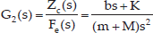
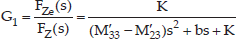
As mentioned before, a simple PD controller could achieve the control of the x coordinate of the leg, but we mainly concentrate on how to control the height of the leg. After Equation (11) has been obtained, the design of the control law in the vertical direction is similar to that presented in Section 3.1. Because F_Ze = -Kr, the transfer function between F_Ze and F_Z is:

${\mathrm{G}}_1=\frac{{\mathrm{F}}_{\mathrm{Z}\mathrm{e}}(\mathrm{s})}{{\mathrm{F}}_{\mathrm{Z}}(\mathrm{s})}=\frac{\mathrm{K}}{({{\mathrm{M}}^{\prime }}_{33}-{{\mathrm{M}}^{\prime }}_{23}){\mathrm{s}}^2+\mathrm{b}\mathrm{s}+\mathrm{K}}$

(12)

Then the force control law of inner loop is as follows:

${\mathrm{F}}_{\mathrm{Z}}={\mathrm{F}}_{\mathrm{Z}\mathrm{d}}+{\mathrm{K}}_{\mathrm{F}}({\mathrm{F}}_{\mathrm{Z}\mathrm{d}}-{\mathrm{F}}_{\mathrm{Z}\mathrm{e}})-({{\mathrm{M}}^{\prime }}_{33}-{{\mathrm{M}}^{\prime }}_{23})\mathrm{g}$

(13)

where F_Ze is the force between the leg and ground in the vertical direction, which could be measured through the force sensor installed on the foot.

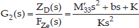
Due to M₃₁ ã 0, the transfer function between Z_D and F_Ze is:

${\mathrm{G}}_2(\mathrm{s})=\frac{{\mathrm{Z}}_{\mathrm{D}}(\mathrm{s})}{{\mathrm{F}}_{\mathrm{Z}\mathrm{e}}(\mathrm{s})}=\frac{{{\mathrm{M}}^{\prime }}_{33}{\mathrm{s}}^2+\mathrm{b}\mathrm{s}+\mathrm{K}}{\mathrm{K}{\mathrm{s}}^2}$

(14)

The whole control process is shown in Figure 6.

Figure 6.

Control block diagram

If taking the gravity into consideration, the position control law is as in Equation (15):

$\begin{array}{l}{{\mathrm{F}}^{\prime }}_{\mathrm{X}\mathrm{d}}={\mathrm{K}}_{\mathrm{p}\mathrm{x}}({\mathrm{X}}_{\mathrm{D}\mathrm{d}}-{\mathrm{X}}_{\mathrm{D}})+{\mathrm{K}}_{\mathrm{d}\mathrm{x}}({\dot{\mathrm{X}}}_{\mathrm{D}\mathrm{d}}-{\dot{\mathrm{X}}}_{\mathrm{D}})+{\ddot{\mathrm{X}}}_{\mathrm{D}\mathrm{d}}+{{\mathrm{M}}^{\prime }}_{13}\mathrm{g}\\ {{\mathrm{F}}^{\prime }}_{\mathrm{z}\mathrm{d}}={\mathrm{K}}_{\mathrm{p}\mathrm{z}}({\mathrm{Z}}_{\mathrm{D}\mathrm{d}}-{\mathrm{Z}}_{\mathrm{D}})+{\mathrm{K}}_{\mathrm{d}\mathrm{z}}({\dot{\mathrm{Z}}}_{\mathrm{D}\mathrm{d}}-{\dot{\mathrm{Z}}}_{\mathrm{D}})+{\ddot{\mathrm{Z}}}_{\mathrm{D}\mathrm{d}}+{{\mathrm{M}}^{\prime }}_{33}\mathrm{g}\end{array}$

(15)

4. Simulation Analyses

4.1 One-dimensional Model simulation

Section 3.1 presents the control algorithm of the one dimensional model. On the assumption that the parameters in section 3.1 are setted as Table 1 shows

Table 1.

Parameters of the one dimensional model

parameter
M	45kg
m	5kg
K	61000N/m
b	1104.5N/m/s

In addition, assume that k_p and k_d respectively are 0.2K and 0.02K. The simulation results are shown in Figure 7 and Figure 8.

Figure 7.

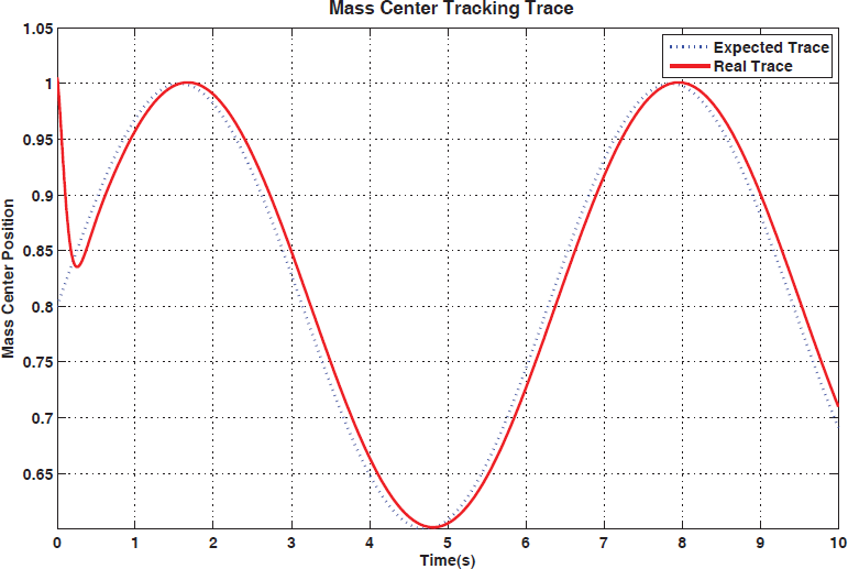
Mass centre tracking trace when K=61000

Figure 8.

Force from the ground when K=61000

On the other hand, taking K=610000 as stiff contact between foot and ground. The simulation results are shown in Figure 9 and Figure 10. According to the comparison between these two kinds of results, we can learn that the control algorithm proposed in Section 3.1 has a smaller contact force and a better tracking trace.

Figure 9.

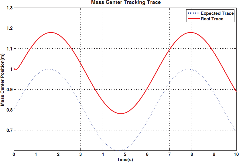
Mass centre tracking trace when K=610000

Figure 10.

=Force from the ground when K=610000

4.2 Multidimensional Single Leg Simulation

Suppose the parameters of the single leg as shown in Table 2.

Table 2.

Parameters of the single leg

Param.	Length/m	Mass/kg	Moment of inertia/kg ṁ m2
Rod
1	−	20.0	0
2	0.25	3.50	0.07
3	0.30	3.00	0.09
4	0.30	2.50	0.07

The coefficient α = 0,β = 0 and the gain coefficients K_px and K_dx are set as 3000 and 100, respectively. K_pz and K_dz are set as 3000 and 250, respectively. K_F is set as 4. To verify the proposed algorithm when controlling height of the single leg, input a sinusoid in vertical direction as desired trace. The simulation results in MatLab are shown in Figure 11, Figure 12 and Figure 13.

Figure 11.

Height of leg

Figure 12.

Tracking in vertical direction

Figure 13.

Tracking error in vertical direction

We can learn from Figure 12 that the leg could track the sinusoid well after a control time of about 100ms. The real trace has a delay of about 6ms at most, compared to the expected trace.

We can learn from Figure 13 that the tracking error curve is a sinusoid, whose cycle is the same as the expected input sinusoid. We can also discover that the maximum error is less than 8mm.

5. Conclusions

In this paper, we take a single leg of the quadruped robot as a research object and discuss the control law in the operation space. First, we establish the joint space model and then establish the operation space model. Next we design the control law (named PCWIFL) in the operation space and verify the controller through simulation in Matlab.

Consequently, we can learn from the simulation results that the leg could track the given trace well with the controller designed in this paper. It indicates that the controlling algorithm can meet the requirements within the allowed range basically.

A quadruped robot is designed to walk on complex ground. Force control is significant for adapting to the environment. Moreover, research on how to make the best of the feedback force of the foot, in order to reach compliance control of the leg has good prospects.