Sage Journals: Discover world-class research

Abstract

Estimation of distribution algorithms (EDAs), as an extension of genetic algorithms, samples new solutions from the probabilistic model, which characterizes the distribution of promising solutions in the search space at each generation. This paper introduces and evaluates a novel estimation of a distribution algorithm, called L1-regularized Bayesian optimization algorithm, L1BOA. In L1BOA, Bayesian networks as probabilistic models are learned in two steps. First, candidate parents of each variable in Bayesian networks are detected by means of L1-regularized logistic regression, with the aim of leading a sparse but nearly optimized network structure. Second, the greedy search, which is restricted to the candidate parent-child pairs, is deployed to identify the final structure. Compared with the Bayesian optimization algorithm (BOA), L1BOA improves the efficiency of structure learning due to the reduction and automated control of network complexity introduced with L1-regularized learning. Experimental studies on different types of benchmark problems show that L1BOA not only outperforms BOA when no prior knowledge about problem structure is available, but also achieves and even exceeds the best performance of BOA that applies explicit controls on network complexity. Furthermore, Bayesian networks built by L1BOA and BOA during evolution are analysed and compared, which demonstrates that L1BOA is able to build simpler, yet more accurate probabilistic models.

Keywords

Estimation of Distribution Algorithms Evolutionary Computation Bayesian Optimization Algorithm L1-Penalized Regression Bayesian Networks

1. Introduction

Estimation of distribution algorithms (EDAs) [1], also called probabilistic model building genetic algorithms (PMBGAs) [2], have been recently identified as a novel paradigm in the field of evolutionary algorithms (EAs). Unlike traditional EAs, such as a simple genetic algorithm (sGA) [3], EDAs replace classical genetic operators (e.g., mutation or crossover) by building and sampling probabilistic models of promising candidate solutions.

EDAs ensure an effective mixing and reproduction of promising partial solutions, thereby solving GA-hard problems with linear or subquadratic performance in terms of fitness function evaluations [4].

According to the modelling of interactions between variables of optimization problems, two families of EDAs have been proposed. The first one, called univariate EDAs, assume that variables in a problem are independent of one another and, hence only a product of independent univariate probabilities is served as the distribution of promising solutions. Univariate EDAs include the univariate marginal distribution algorithm (UMDA) [5], the compact genetic algorithm (CGA) [6], population-based incremental learning (PBIL) [7], etc. This class of EDAs is known for its simplicity and computational efficiency in model learning. However, the inability to solve problems where nonlinear interactions among variables exist prevents those algorithms from solving a broader class of problems. Later developments in EDAs leverage joint distributions of variable pairs or groups to model multivariate interactions and achieve a very good performance on a wide range of decomposable problems. These algorithms include the factorized distribution algorithm (FDA) [8], the extended compact genetic algorithm (ECGA) [9], the estimation of Bayesian network algorithm (EBNA) [10] and the Bayesian optimization algorithm (BOA) [11][12], to name a few.

As one of the state of the art multivariate EDAs, BOA [11][12] uses Bayesian networks [13] to capture the dependencies between the decision variables of the problem. Obviously, the structural accuracy of the Bayesian network learned during each generation significantly impacts the quality of the solutions and the efficiency of the evolution. Unfortunately, it is an NP-hard problem to extract the optimal structure of a Bayesian network given a set of data, regardless of the size of the data [14]. BOA uses a greedy strategy, called score + search, to learn the structure from promising solutions. The strategy performs a search through the space of possible structures with a scoring function, such as Bayesian information criterion (BIC) [15] or the Bayesian - Dirichlet (BD) metric [16], measuring the fitness of each structure. The structure achieving the highest score is then selected. It has been pointed out in [17] that BIC often results in overly simple models and requires large populations to learn a model that captures all necessary dependencies. On the other hand, BD tends to generate an overly complex network due to the existence of noises. Consequently, an additional parameter is added to specify the maximum order of interactions between nodes and to quit structure learning prematurely [12]. As noted in [18], the choice of the upper bound on the network complexity strongly affects the performance of BOA. However, the proper bound value is not always available for black box optimization.

In this paper, a new estimation of distribution algorithm, L1-regularized Bayesian optimization algorithm (L1BOA) is proposed. In spite of relying on Bayesian networks to model distribution of promising solutions, we first utilize L1-regularized logistic regression to identify the potential dependencies between variables firstly. The idea is to apply regression analysis for each variable on the other ones and the regression coefficients with relatively large absolute values are explained as edges in the Bayesian network. Since L1-regularized regression gives exactly zero regression coefficients to most irrelevant or redundant variables [19], it provides a powerful tool for finding the candidate parents of each variable, which leads to a sparse but nearly optimized network structure. Then, greedy search, which is restricted to candidate parent-child pairs, determines the final structure of the network. Due to the excellent properties of L1-regularized learning, L1BOA not only controls the complexity of the network automatically and efficiently, according to the nature of the problem to be solved, but also learns the network structure efficiently with a smaller population size.

To evaluate our new algorithm, two sets of experiments between L1BOA and BOA are performed on different types of test functions, where two cases of BOA, i.e., with and without artificial bounds on network complexity, are considered respectively. The results indicate that the bounds play a key role in the performance of BOA and L1BOA always achieves, even exceeds, the performance of BOA with optimal complexity bounds. Furthermore, we compare the accuracy and the complexity of probabilistic models (i.e., Bayesian Networks) built by L1BOA and BOA based on the perfect models of the test functions. The empirical results of model investigations show that L1BOA is able to build simpler yet more accurate models and there is a positive correlation between performance of the algorithm and accuracy of the model it builds.

The remainder of this paper is organized as follows. In Section 2, some background materials are introduced. Section 3 describes L1BOA in detail. The experimental setup is illustrated in Section 4, followed by Section 5, which compares the performances of L1BOA and BOA. In Section 6, probabilistic models (i.e., Bayesian Networks) built by L1BOA and BOA are investigated. Section 7 discusses the merit of L1BOA. Finally, the paper is summarized in Section 8.

2. Related Work

2.1 Bayesian Networks

Bayesian networks [13] are powerful graphical models that combine probability theory with graph theory to encode probabilistic relationships between variables. A Bayesian network is defined by its structure and corresponding parameters. The structure is represented by a directed acyclic graph where the nodes correspond to the random variables to be modelled and the edges correspond to conditional dependencies. (Throughout our paper, the terms node and variable are used interchangeably.) The parameters are represented by a set of conditional probability tables (CPTs), which specify the conditional probabilities for each variable with all possible instances of the parent variables. More formally, the factorization of the joint probability distribution in a Bayesian network is defined as

p (X) = Π_{i = 1}^{n} p (X_{i} | X_{p a_{i}})

(1)

where X = (X₁, X₂,…,X_n) denotes a vector of random variables, X_pai refers to the set of parents of X_i and p(X_i | X_pai) is the conditional probability of X_i given the parents X_pai.

2.2 Bayesian Optimization Algorithm

As one of the multivariate EDAs, the Bayesian optimization algorithm (BOA) [11][12] generates a population of candidate solutions by building and sampling Bayesian networks. After the initialization of a population at random, with a uniform distribution over all possible solutions, the population is then updated for a number of generations. In each generation, BOA works as follows: (1) promising solutions are selected from the current population by means of a selection method, such as tournament or truncation selection; (2) the structure of a Bayesian network that models the population of promising solutions is constructed; (3) the conditional probabilities of the Bayesian network are identified according to promising solutions; (4) the offspring population is generated by sampling the built Bayesian network; (5) replacement scheme is executed to incorporate new solutions into the original population. The above five steps are repeated until some termination criteria are satisfied.

To build a Bayesian network from the promising population, both the structure and the CPTs have to be learned. BOA adopts a greedy strategy to learn the structure of Bayesian networks. More specifically, a certain score of the network is employed to measure the quality of Bayesian network structures. At the beginning, the network is initialized as an empty network with no edges. Then the edge that improves the network score most is added in each step, until no further improvement is possible. Additionally, the number of edges that end in any node is usually limited to some artificial bound to control the complexity of the final structure [12]. After the structure is learned, the calculation of CPT for each variable corresponds to counting the number of times that each possible value of the variable appears, given all possible values of its parents in the promising population.

2.3 Graphical Model Learning using L1-Regularization

Traditionally, learning the structure of graphical models is viewed as a combinatorial search problem. In recent years, solving the problem using L1-regularized learning has been proposed [20, 21, 22, 23, 24]. In such a way, the structural learning is embedded within the problem of parameter estimation. To prevent overfitting, regularization is a common technology, which adds an extra term in the regression (linear or logistic) to penalize models using a large number of features. In a variety of regularization technologies, it is known [19] that L1-regularization, in which the penalty term is formed as the absolute values of the parameters, tends to lead to sparse models, where many weights have value zero. Features that have a weight of zero do not induce dependencies between the variables they involve. Consequently, it is able to estimate parameters and select variables simultaneously. Moreover, it has been shown that L1regularization has a logarithmic sample complexity [25], which means that the number of samples required learning a proper structure grows only in proportion to the logarithm of the problem size. For EDAs that means a small population size for global convergence, as will be shown in our experiments. Therefore, L1-Regularization provides a competitive alternative in learning the structure of graphical models.

3. Structure Learning for L1BOA

This section presents our method of learning structure for LIBOA. As outlined in Algorithm 1, L1BOA consists of generations including the same five steps as BOA [11][12] (see Section 2.2). The main peculiarity of L1BOA, with respect to BOA, lies in the procedure of learning Bayesian networks by means of L1-regularization (see line 5 in Algorithm 1), which will be discussed in detail as follows.

Algorithm 1

L1BOA

1 t ← 0 2 P_t ← Generate initial random population 3 repeat 4 S ← Select promising individual in P_t 5 B ← L1-regularized Bayesian networks learning from S 6 Learn the condition probability tables of B from S 7 T ← Sample from B 8 P _t₊₁ ← Replace P_t with T 9 t ← t + 1 10 until t > t_max or population converge

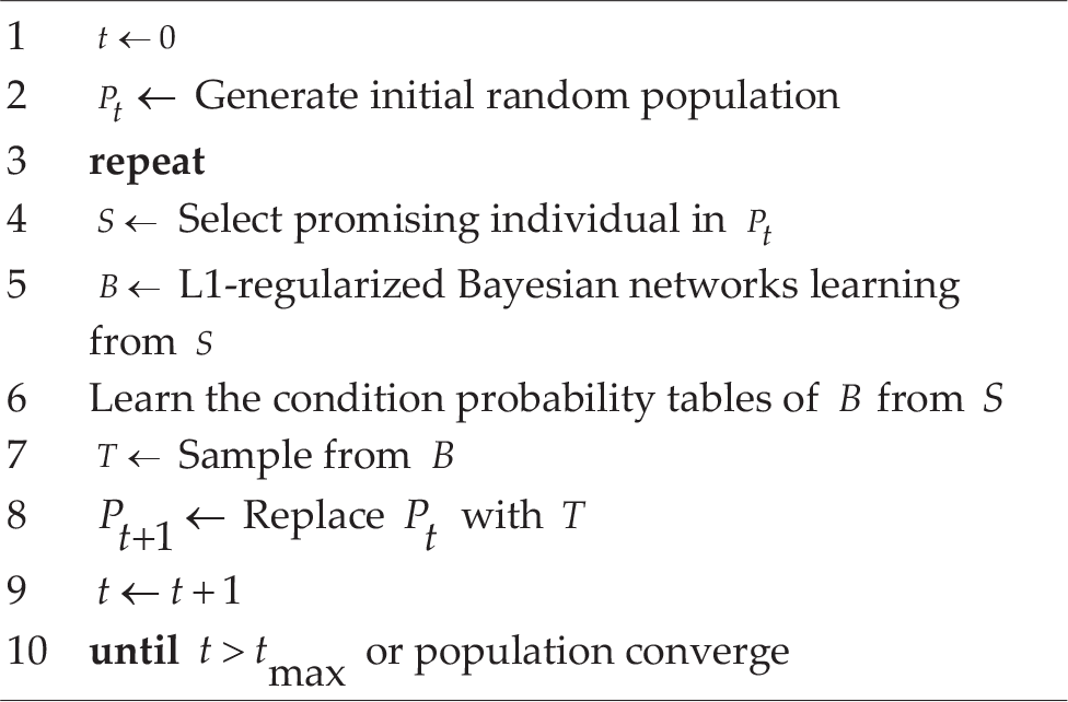
There are two steps in learning the structure of Bayesian networks via L1-regularization. In the first stage, each variable is applied by L1-regularized logistic regression on the other ones and the non-zero elements in regression coefficients identify the candidate parents of the variable. In the second stage, a greedy search is only restricted to edges in candidate parent-child pairs. Before describing the two steps above, we first discuss how to form the problem of learning the structure of a Bayesian network as a penalized logistic regression problem.

3.1 Problem Setup

The goal of structure learning, given the promising population, is to find the Bayesian network B that maximizes the Bayesian information criterion (BIC) score [15], or equivalently minimizes the minimum description length (MDL) cost [26], defined as

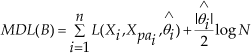
M D L (B) = Σ_{i = 1}^{n} L (X_{i}, X_{p a_{i}}, \overset{\land}{θ_{i}}) + \frac{| \overset{\land}{θ_{i}} |}{2} \log N

(2)

where n specifies the number of variables (i.e., the length of the bits representing candidate solutions), N is the size of the training data set (i.e., the size of the promising population), X_pa are the parents of variable X_i in the network, $L (X_{i}, X_{p a_{i}}, \overset{}{{\hat{θ}}_{i}})$ denotes to the negative log-likelihood of i variables X_i with parents X_pai and parameters θ_i, θ_i = argmin θ L(X_i, X_pai, θ_i) refers _i to the maximum likelihood estimate of X_i 's parameters and | θ_i | is the number of free parameters (i.e., the number of non-zero elements in θ_i) in the CPTs for variable X_i. The negative log-likelihood i of variables X_i is defined as

L (X_{i}, X_{p a_{i}}, \overset{\land}{θ_{i}}) = \underset{x_{i}, X_{p a_{i}}}{Σ} \log p (x_{i} | x_{p a_{i}}, θ_{i})

(3)

Here X_i and π_i are the instances of X_i=x_i and ∏_i = π_i in the training data set, respectively. For binary problems, the logistic regression model [27] is usually used to turn linear predictions into probabilities. Given its parents X_pa, the probability distribution of X_i is defined as follows.

\begin{array}{l} p (x_{i} | x_{p a_{i}}, θ_{i}) = σ (X_{i} (θ_{i} ​^{* T} X_{p a_{i}} + θ_{i_{0}})) \\ = \frac{1}{1 + \exp (- X_{i} (θ_{i} ​^{* T} X_{p a_{i}} + θ_{i_{0}}))} \end{array}

(4)

where X_i ∈{–1, +1}_* and θ_i, which includes bias θ_i₀ and non-bias term θ_i = (θ_i1,θ_i2,…), denote the regression coefficients in the lo gistic regression model. And σ(a) is the logistic sigmoid function defined by

σ (a) = \frac{1}{1 + \exp (- a)}

(5)

To compute the maximum of equation (3), while reducing the variance of the estimates and preventing overfitting, an L1 penalty term is added to form the L1-regularized logistic regression, which is defined as the following.

\overset{\land}{θ_{i}} (λ, X_{p a_{i}}) = \arg \min_{θ_{i}} L (X_{i}, X_{p a_{i}}, θ_{i}) + λ | | θ_{i} ​^{*} | |_{1}

(6)

where the parameter λ>0, called regularizer, governs the relative importance of the regularization on the non-bias term of regression coefficients, compared with the likelihood. L1-regularization has the property that if regularizer A is sufficiently large, some elements in the non-bias term of i (i.e, i) are driven to zero, leading to a sparse model in which the corresponding variables in the model play no role [19]. Consequently, such a technique provides a powerful strategy to select candidate parents of each variable from X_pai.

In equations (4) and (6), the variable X_i is applied to a logistic regression on the variables in X_pai. Therefore, the absolute value of each element in a non-bias term of regression coefficients θ_i reflects the strength of the dependency between the corresponding variable and X_i. The greater the absolute value, the stronger the dependency. On the other hand, since a larger regularrer makes many of the elements in θ_i zero, the set X_pai including the variables whose corresponding parameter i s in non-bias terms of θ_i are non-zero (i.e., $\overset{\land}{X_{p a_{i}}} = {X_{j} ∣ j \in \emptyset}$ , could be regarded as the candidate parents of X_i.

3.2 Candidate Parents Detection

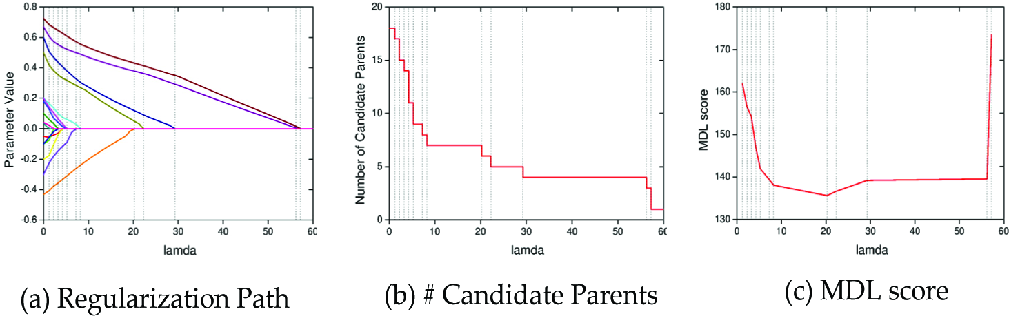
From the discussion above, the problem of detecting the candidate parents is shifted to determine a suitable value of the regularizer λ. In equation (6), candidate parents of each node could be seen as a function of λ. The family of solutions as Avaries over (0,+∞) forms the regularization path. The stronger regularizer leads to more elements in the non-bias term of θ_i zero, thus selecting fewer candidate parents. Figure 1 (a) represents the impact of the regularizer on the value of each element in θ_i except bias θ_i0, in which the values of different elements are represented by solid lines with different colours. The changes in the number of candidate parents and MDL score as the regularizer varies are represented in Figure 1 (b) and (c) respectively. The vertical dash lines in Figure 1 demonstrate that some elements in the regression coefficient are not equal to zero any more when the lines are lower than the corresponding value on the horizontal axis. In such a situation, it means that some new candidate parents emerge.

Figure 1.

The impacts of the regularizer (i.e., λ) are represented when applying L1-regularized logistic regression.

A naive approach available is to use the same λ for all nodes. However, such an approach has three drawbacks. First, different problems produce different types of dependencies between variables. Fixing the value of λ weakens the robustness of the algorithm. Second, as the scale of some separative problems increases, the structure of the whole problem changes, even if the dependencies between different variables remain the same. Third, in asymmetrical problems, some variables in real structure may depend on more variables than others. In fact, using a uniform value produces the same disadvantages as the one generated by treating the maximum income edges as a constant in BOA [11][12].

To determine λ, cross-validation is the typical approach. However, the process is quite time consuming since the approach would have to be applied on each node. In [21] the number of non-zero elements in non-bias terms of θ_i (i.e., the number of candidate parents) is piecewise constant against λ, with kinks at each point where any element transitions from zero to non-zero, or vice versa (see Figure 1(b)). Hence, a searching approach with n steps along the regularization path [21] is utilized in this paper. The procedure begins with λ = λ₀, which is the minimum value making all elements in θ_i zero except bias 0. The value of 0 is equal to the maximum gradient magnitude when all non-bias parameters are zero (i.e., θ_i* = 0), and the bias parameters, θ_i0 is at its optimal value, since all larger values of λ will have inactive non-bias parameters. Then a fixed step length δλ = λ_k – λ_k+1 = λ / n is taken to decrease the value of λ. In step k, the maximum likelihood parameters θ_i are computed according to the current value of the regularizer k. MDL score could be calculated according to equation (6). If the MDL score is improved, the set of variables, whose corresponding parameters in θ_i are non-zero, are recorded as the candidate parents of that node. Finally, the set achieving the minimum MDL is treated as the candidate parents.

Algorithm 2 CandParents(Xi, Xpai)

1. λ ← The minimum value making all parameters in

{\hat{θ}}_{i}

zero 2.

{\hat{θ}}_{i} \leftarrow arg {min}_{θ_{i}} L (X_{i}, X_{p a_{i}}, θ_{i}) + λ_{0} ∣ ∣ θ_{i} ∣ ∣_{1}

M D L_{min} \leftarrow L (X_{i}, X_{p a_{i}}, {\hat{θ}}_{i})

4. k ← 0 5. δ_λ = λ₀ / n 6. while k<n do 7. k ← k + 1 8. k ← k + 1 9. λ_k λ_{k + 1} – δ_λ 10.

M D L_{min} \leftarrow L (X_{i}, X_{p a_{i}}, {\hat{θ}}_{i})

11 if MDL<MDL_min then 12

\emptyset = {z ∣ θ_{i z} \neq 0, z \neq 0}

X_{p a_{i}}^{^} = {X_{j} ∣ j \in \emptyset}

14 end if 15 end while 16 return X^{^}_pai

As noted before, the number of candidate parents is piecewise constant against λ, and increases only at the value of λ where some elements in regression coefficients change from zero to non-zero (see the vertical dash lines in Figure 1). Therefore, the optimal MDL score must be achievable at these points and it is sufficient to check O(n) values of λ along the path to find the candidate parents of each variable, where n is the number of nodes in network. Furthermore, O(Nn²) is needed for each step in the regularization path to compute maximum likelihood estimates of the logistic regression using iteratively reweighted least squares (IRLS) [28]. Hence, the complexity of computing the candidate parents of each node is O(Nn³), where N denotes the size of the training data set. The procedure of finding candidate parents by tuning the regularizer is described in Algorithm 2.

3.3 Pruned Network Search

In equation (6), it is notable that X_pai also influences the detection of the candidate parents of each node. There are several different ways to construct X_pai. One of the choices is to leverage the order search. Using hill climbing to find the best order of all nodes [29], X_pai could consist of the precedents before node X_i according to the ordering. In such a case, the cardinality of X_pai is equal to the number of precedents of X_i, thus $X_{p a_{i}}$ . In this paper, we set $X_{p a_{i}} = (X_{1}, X_{2}, ..., X_{i - 1}, X_{i + 1}, ..., X_{n})$ , thus $ ∣ X_{p a_{i}} ∣ = n - 1$ . Th pa s means that each node apples regression i on the others to identify the candidate parents according to the procedure described in Section 3.2.

Algorithm 3 L1-regularized Bayesian Networks Learning

1. Initialize an empty Bayesian network B 2. for each variable X_i in the problem do 3.

X_{p a_{i}} \leftarrow (X_{1} - X_{2}, \dots, X_{i - 1}, X_{i + 1}, \dots, X_{n})

X_{p a_{i}}^{^} \leftarrow C a n d P a r e n t s (X_{i}, X_{p a_{i}})

5. end for 6.

E \leftarrow All edges within pairs {(X_{j}, X_{j}) ∣ X_{j} \in X_{p a_{i}}}

7. repeat 8. e ← Select the edge from E improving MDL most 9. E ← E –{e} 10. Add e into B 11. until MDL(B) is not improved or E is empty 12. return B

To add actual edges into the network, there is another issue to be considered. Since the dependencies may be asymmetric in the finite sample scenario (for example, the edge X₁ - X₂ may be found when regressing on X₁ but not on X₂), two strategies, called ‘OR’ and AND’ had to be chosen In the former, X_i is selected as the candidate parent of X_j if either the dependency X_i - X_j or X_j - X_i is detected j In such a strategy, X₂ is selected as the candidate parent of X₁ and vice versa, since the dependency X₁-X₂ is detected when regressions are applied for X₁. The latter strategy chooses candidate parents when the both directions are identified, which means X₂ is not selected as the candidate parent of X₁, even though the dependency X₁-X₂ is detected. Because the discrepancies between the two strategies are not remarkable [30] the ‘OR’ strategy is used in this paper. The reason lies in that the procedure is to find a set of variables with all the parents, children and co-parents, ideally only discarding false parents and our goal is to identify which edges to leave out, rather than which edges to include. Consequently, the cost of excluding a true edge is higher than including a spurious edge and each edge forms two candidate parent-child pairs to be considered in the greedy search.

Once the candidate parents of each node are known, the greedy search, which is restricted to these node pairs, is employed to make the final decision about which edges to include. Since L1-regularization is proved to hold a parsimonious property [31], the candidate detection usually reduces the search space quite a lot. The details about Bayesian networks structure learning via L1-Regularization are presented in Algorithm 3 and line 4 in Algorithm 3 has been described in Algorithm 2.

4. Experimental Setup

4.1 Test Functions

To compare the performance of L1BOA and BOA, the experiments on four additively decomposable test functions are performed. Function Onemax:

f_{o n e \max} (x) = u (x) = Σ_{i = 1}^{n} x_{i}

(7)

where x_i represents the ith bit of the input string with length n. More 1s in the solution are included, the higher the fitness becomes. The optimum, equal to n, is achieved in the string of all ones. In Onemax, there are no dependencies between variables. Function Link-10:

f_{l i n k 10} (x) = \sum_{i = 1}^{n ∕ 10} l i n k 10 (x_{10 i - 9} x_{10 i - 8} ... x_{10 i})

(8)

where

l i n k 10 (x_{10 i - 9} x_{10 i - 8} ... x_{10 i}) = Σ_{j = 1}^{4} t_{j} + v + u

(9)

{\begin{cases} t_{j} = {\begin{cases} 1, & i f x_{10 i - 2 j - 1} = x_{10 i - 2 j} \\ 0, & o t h e r w i s e \end{cases} ​ (10) \\ u = {\begin{cases} 1, & i f x_{10 i - 1} \neq mod (Σ_{j = 1}^{4} x_{10 i - 2 j}, 2) \\ 0, & o t h e r w i s e \end{cases} ​ (11) \\ w = {\begin{cases} x_{10 i}, & i f Σ_{j = 1}^{4} x_{10 i - 2 j - 1} = 4 \\ 0 & o t h e r w i s e \end{cases} ​ (12) \end{cases} ​

(10)

In Link-10, the input string is first partitioned into independent groups of 10 bits each. Equations (10), (11) and (12) are applied to each group. The contributions of all the groups are added together to form the fitness. The optimum of n-bit Link-10 is 0.6n, which is achieved in the string of all ones. The dependencies between variables in Link-10 are sparse and asymmetrical. More specifically, x_10i and x_10i−1 depend on more variables than others in each group. Consequently, Link-10 is just an example of the asymmetrical problem mentioned in Section 3.2. Function Uniformly Scaled Trap-4 [32]:

f_{t r a p_{​_{4}}} (x) = Σ_{i = 1}^{n ∕ 4} t r a p_{​_{4} (x_{4 i - 1} x_{4 i - 2} x_{4 i - 3} x_{4 i})}

(13)

t r a p_{4} (u) = {\begin{cases} 4, i f u = 4 \\ 3 - u, o t h e r w i s e \end{cases}

(14)

where u is the number of ones in the input string of 4 bits. The input string in uniformly scaled Trap-4 (uTrap-4) is also partitioned into disjointed groups. Each 4-bit group applies Trap-4 function, which is defined in equation (14).

The fitness is the sum of the contributions of each group. The optimum of n-bit uTrap-4, which is equal to n, is achieved in the string of all ones. It necessitates that all bits in each group are treated together, because lower order statistics lead the search away from the global optimum.

Function Exponentially Scaled Trap-4 [33]:

f_{e t r a p_{​_{4}}} (x) = Σ_{i = 1}^{n ∕ 4} 3^{i} • t r a p_{​_{4} (x_{4 i - 1} x_{4 i - 2} x_{4 i - 3} x_{4 i})}

(15)

Similar to uTrap-4, equation (14) is applied to each 4-bit group in exponentially scaled Trap-4 (euTrap-4). Rather than treating each group equally in uTrap-4, the contributions to the fitness of each building block are scaled exponentially. Such a scale gives each group distinguishable importance according to its position. Uniformly scaled functions resemble problems with subproblems of equal importance, while exponentially scaled functions represent those with subproblems of distinguishable importance.

4.2 Parameters Settings

In all experiments, both L1BOA and BOA choose truncation selection with ps = 0.5 as the selection strategy. This means that the best half of the current population is selected as promising individuals. We employ truncation selection because tournament selection leads the models in BOA to be overly complex [34] and using truncation is much better for leading to accurate structural linkage information [35]. Since the choice of replacement strategy is not relevant to the performance when using truncation selection [35], we employ simple elitist replacement with pr = 0.5, in which the worst 50% of the population are replaced by newly generated solutions. Forward sampling of Bayesian networks [13] is adopted in both L1BOA and BOA to generate offspring in each generation. In addition, both algorithms are terminated when the population converges on the global optimum (success) or when the upper bound on the number of generations has been reached (i.e., t>_max in Algorithm 1) without discovering the global optimum (failure). Unless otherwise specified, the maximum generations tmax is set as 200. The parameters described above are listed in Table 1.

Table 1.

Parameters Settings

	Strategy	Parameter
Selection	Truncation Selection	ps = 0.5
Sample	Forward Sample
Replacement	Elitist Replacement	pr = 0.5
Termination	Convergence or t>t_max	t_max =200

5. Performance Comparison

In this section, two sets of experiments are conducted to compare the behaviours of L1BOA and BOA. The BD metric with K2 prior [16] is used to construct the Bayesian network in BOA in both sets, because BIC often results in overly simple models and requires large population to learn a model [17]. In the first set of experiments, the procedure of network structural learning in BOA is terminated only when the score is not improved. Then, the bound on the complexity of networks is treated as an additional criterion to end the network structural learning in BOA. When the number of edges added into the network excesses the bound, the structural learning stops early. Furthermore, various values of bound are taken into account to investigate how that parameter impacts on the performance of BOA.

5.1 Comparison between L1BOA and BOA without Complexity Control

The performance comparison between L1BOA and BOA without extra network complexity control is represented in this subsection. The problem sizes of three test functions are all set at 40 and population sizes are augmented by the power of 2. Two metrics are calculated to evaluate BOA and L1BOA: (1) the fitness, which is equal to the final result algorithms converging to; (2) the success rate (S.R.), which is set as the ratio of successful runs to total runs. The experimental results are depicted in Figure 2, where fitness and success rate are under the scale of left Y-axis and right Y-axis, respectively. As can be noted from Figure 2, the fitness of L1BOA is higher than that of BOA in all test functions with the same population size. The gaps in fitness between L1BOA and BOA are remarkable. From the aspect of success rate, BOA is able to find the global optimum of Onemax, but needs a larger population than L1BOA. For function uTrap-4, although BOA could converge to the global optimum sometimes (about 60% of the time), it is not able to ensure the convergence in each run. This means that BOA could not find enough linkages in all the groups. A similar situation emerges with function eTrap4. As the population rises, the success rate falls, which implies that BOA could not converge on the optimum of eTrap4. Things are even worse when BOA deals with Link-10. It could hardly find the global optimum of Link-10 for the success rate nearly stays at zero. On the other hand, L1BOA could converge on the global optimum of Link-10 in all the runs with a relatively smaller population.

Figure 2.

Performance comparison between L1BOA and BOA without artificial control on network complexity.

From the results above, it could be concluded that network complexity control is necessary for BOA in addition to the K2 criteria that are normally used. Without the bound, BOA could not converge on the global optimal when handling problems with dependencies between variables. It is also obvious that L1BOA outperforms BOA without such a bound.

5.2 Comparison between L1BOA and BOA with Complexity Control

This subsection describes the performance comparison between L1BOA and BOA. The complexity of a network is restricted by the maximum number of income edges per node, denoted as k in the rest of this paper. We discuss two aspects of the performance, including the required minimum population size (RMPS) and interrelationship between population sizes and generations.

5.2.1 Comparison on Population Requirements

Here, we focus on the population requirements of L1BOA and BOA with different values of k. The ranges of the problem sizes are represented in Table 2. For each case of different functions, the RMPS to ensure the algorithm converges in all 30 runs is determined empirically by a bisection method [12]. Furthermore, the function evaluations are also compared when population sizes are set as the RMPS. The function evaluations of each case are calculated as the average over 30 runs with a 95% confidence interval.

Table 2.

Problem Sizes of Test Function

Function	Range of Problem Sizes
Onemax	{30, 40, 50, 60, 70, 80}
Link-10	{30, 40, 50, 60, 70, 80}
uTrap-4	{32, 40, 48, 56, 64, 72}
eTrap-4	{32, 40, 48, 56, 64, 72}

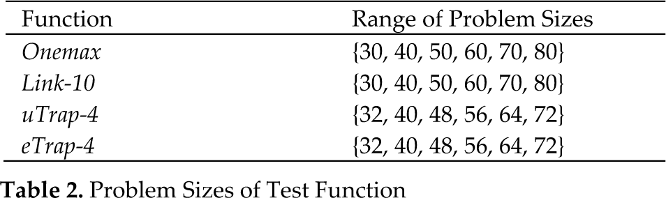
Figure 3(a) shows the empirical results of population requirements of Onemax. Obviously, BOA with k = 0 is able to rely on the lowest RMPS to converge on the optimum in all the instances. The RMPS of L1BOA are a little higher than those of BOA with k = 0, but remarkably they are lower than those in the other cases (e.g., BOA with k = 1, 2, 3). It is also notable that as the value of k increases, a larger population is needed to enable BOA to converge on the optimum. The same situation is observed in Figure 4(a), which represents the function evaluations of L1BOA and BOA on Onemax.

Figure 3.

Performance comparison on required minimum population size between L1BOA and BOA with network complexity control.

Figure 4.

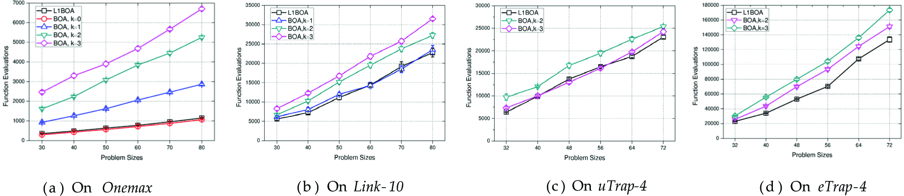
Performance comparison on the number of function evaluations between L1BOA and BOA with network complexity control.

The comparison of the population requirements of Link-10 is depicted in Figure 3(b). The RMPS required by L1BOA are lower than those in all BOA cases. This grows when the value of k increases within BOA. It is worth pointing out that BOA with k = 0 needs a population and function evaluations one order of magnitude larger than the other cases to converge on the global optimum. Figure 4(b) demonstrates that the corresponding function evaluations of L1BOA are nearly the same as that of BOA with k = 1 and the trend of function evaluations of BOA with various bounds are identical to the situation of population requirements. Figure 3(c) and Figure 4(c) depict the experimental results of uTrap-4. BOA with k = 0, 1 is not able to achieve the global optimum of uTrap-4 since the problem necessitates that bits in each group are treated together. Because each group consists of four bits, k = 3 allows every bit to link with all the others in the same group. Consequently, only the cases with k equal to 2 and 3 are taken into consideration. It has been seen that the RMPS and the corresponding function evaluations of L1BOA are equal to those of BOA with k = 3 overall and are apparently lower than those of BOA with k = 2.

Groups in eTrap-4 are applied in the same function as uTrap-4. L1BOA is compared with BOA with k = 2, 3 in eTrap-4 as well. In Figure 3(d), L1BOA relies on the lowest RMPS to converge on the optimum in all cases. Within BOA, the RMPS of case k = 2 is less than that of k = 3, which is the opposite of the situation in uTrap-4. The same trend is also observed in Figure 4(d), which represents the function evaluations of L1BOA and BOA in eTrap-4 respectively. This is because the distinguishable importance of each group degrades the average order of statistics necessary to converge on the global optimal.

Furthermore, we want to test the null hypothesis that the number of evaluations of BOA with different complexity bounds are lower than that of L1BOA. If the hypothesis is accepted, it means that BOA outperforms L1BOA. Since the obtained results may present neither normal distribution nor homogeneity of variance, the Wilcoxon paired signed-ranks test [36], which is a non-parametric test, is executed according to the recommendations made in [37]. The results are presented in Table 3, which validates that L1BOA is able to achieve the performance of BOA with optimally controlled bounds on network complexity, when dealing with uTrap-4 and outperforms BOA when dealing with Link-10 and pTrap-4.

Table 3.

Significance tests on numbers of function evaluations. The p-values are from one sided Wilcoxon paired signed-rank tests.

		R+	R-	p-value
Onemax	BOA(k=0)-L1BOA	21	0	0.0894
	BOA(k=1)-L1BOA	0	21	0.0106
	BOA(k=2)-L1BOA	0	21	0.0106
	BOA(k=3)-L1BOA	0	21	0.0106

Link-10	BOA(k=1)-L1BOA	3	18	0.0468
	BOA(k=2)-L1BOA	0	21	0.0106
	BOA(k=3)-L1BOA	0	21	0.0106

uTrap-4	BOA(k=2)-L1BOA	4	17	0.0711
	BOA(k=3)-L1BOA	0	21	0.0106

eTrap-4	BOA(k=2)-L1BOA	0	21	0.0106
	BOA(k=3)-L1BOA	0	21	0.0106

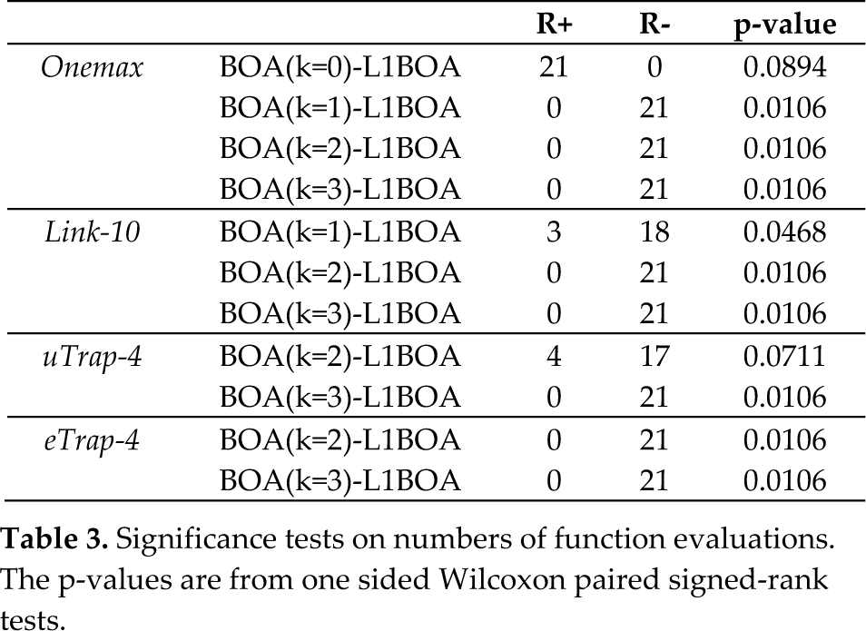
Given the results above, it can be concluded that the network complexity control significantly affects the performance of BOA. Different problems requires BOA to set different bounds to achieve its best performance. On the other hand, the performance of L1BOA is almost equal to, sometimes above, the best in all cases of BOA, when dealing with different functions.

5.2.2 Time-Space Interrelationship

This section describes the behaviour of L1BOA and BOA when the population size increases. The sizes of these three problems are all equal to 40 and the population sizes are increased in proportion to the RMPS estimated in Section 5.2.1. The result of each experiment is calculated as the average over thirty runs with 95% confidence intervals.

Figure 5(a) and Figure 6(a) show the changes in generations and the corresponding function evaluations with increasing population sizes on 40-bit Onemax. In all test cases, the generations of L1BOA are lower than those of BOA no matter what value of k is taken. On the other hand, the generations of L1BOA and BOAs decrease as the population sizes rise. Although the generations reduction of L1BOA is not as notable as those in BOA cases, its function evaluations nearly stay the same, while the increase in function evaluations of BOAs (e.g., k = 1,2, 3) are much more remarkable.

Figure 5.

Performance comparison on the number of generation with the population size increasing.

Figure 6.

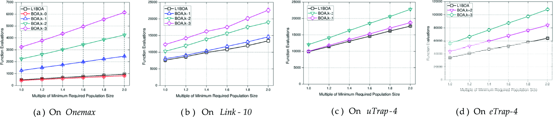
Performance comparison on the number of function evaluations with the population size increasing.

The experimental results on 40-bit Link-10 are depicted in Figure 5(b) and Figure 6(b). The generations of L1BOA are higher than those of BOA, however, its function evaluations remain the lowest in all cases. When a population that is twice as large is used, the function evaluations only increase by one third, which is the lowest in all the cases.

As presented in Figure 5(c), the generations of L1BOA are lower than those of BOA with k = 2, 3 in all cases of 40-bit uTrap-4. Just like the results of Link-10, a decrease in generations is also obtained as the population sizes increase. The only difference is that the generations of L1BOA are reduced more dramatically. In Figure 6(c), when the population size is doubled, the function evaluations of L1BOA increases by less than 50%.

Figure 5(d) and Figure 6(d) show the changes in generations and the corresponding function evaluations when increasing population sizes in 40-bit eTrap-4 function. Although the generations of L1BOA are not the lowest, its function evaluations are always below those of the two cases of BOA when the population is enlarged. Furthermore, the generation's reduction of L1BOA is more remarkable than the two cases of BOA and the function evaluations of L1BOA increase slower than those of two BOA cases.

From the results above, we argue that L1BOA performs as well as, sometimes better than, the best cases of BOA with a larger population available. And the function evaluations of L1BOA grow more slowly when enlarging population sizes.

6. Probabilistic Models Comparison

From the results represented in Section 5, it is already known that the performance of L1BOA is equal to, sometimes above that, of BOA with optimal artificial complexity control. In this section, we investigate the structure of Bayesian networks built by L1BOA and BOA with artificial complexity control. In the investigations, the accuracy and the complexity of the structure are involved. Before comparing Bayesian networks built by L1BOA and BOA, we firstly discuss the perfect models of the test functions according to the relationship between variables in these functions.

6.1 Perfect Models of the Test Function

The test functions used above are all additively decomposable problems. Thus, it is necessary that the probabilistic models encode all or nearly all conditional dependencies between corresponding pairs of variables within each partition. On the other hand, to maximize the mixing and minimize model complexity, it is desirable that we do not discover any dependencies between the different partitions [32] [38].

In Onemax, each bit serves as a building block (BB) and there are no dependencies between these BBs. Consequently, any dependencies in the model are illegal. The perfect model for Onemax is shown in Figure 7 (a). In Link-10, partitions apply equations (10), (11) and (12) to form the fitness. Therefore, the perfect model of Link-10 would obey these equations. According to equation (10), it is clear that there only exists one link for each variable x_10i-k in the same partition when k ≥ 2. (Dependencies only exist between variables if their indexes have the same quotient divided by 2.) On the other hand, equations (11) and (12) show that both x_10i-1 and x_10i depend on a set of variables: the former depends on {x_10i-8, x_10i-6, x_10i-4, x_10i-2} and the latter depends on {x_10i-9, x_10i-7, x_10i-5, x_10i-3}. Therefore, x_10i−1 and x_10i depend on more variables than others. The perfect model of Link-10 in total is depicted in Figure 7 (b), which represents that the necessary dependencies for n-bit Link-10 are 1.2n. Since partitions in both uTrap-4 and eTrap-4 apply 4-bit trap function, the perfect models of them are identical. Trap-4 function, defined in equation (14), is fully deceptive [32]. Therefore, a “perfect” model for solving uTrap-4 and eTrap-4 would contain dependencies between each pairs of bits within the same partition but not contain any dependencies between the different trap partitions. Figure 7(c) depicts the perfect model of uTrap-4 and eTrap-4. The number of necessary dependencies for n-bit of these functions is 1.5n.

Figure 7.

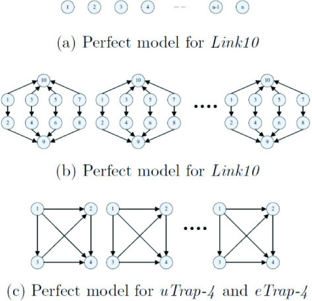
Perfect models for solving Link-10, uTrap-4 and eTrap-4.

According to the discussion above, the distinction between dependencies that should be contained and avoided in the model is straightforward. Consequently, the dependencies that should be included in the perfect model are called necessary dependencies and the dependencies that should be excluded are noted as unnecessary dependencies.

6.2 Accuracy of Probabilistic Models

This subsection discusses the accuracy of the probabilistic models in L1BOA and BOA. Since the perfect model of Onemax contains no dependencies, the accuracies of models are not compared when BOA and L1BOA are dealing with Onemax. For other problems, according to the perfect models discussed above, we investigate the accuracies of dependencies in Bayesian networks built by L1BOA and BOA with explicit complexity control. The accuracies are measured by the average ratio of the number of necessary dependencies to the number of total dependencies in all generations during the evolution. For each experiment case (i.e., each test function with different problem sizes), the population size of BOA and L1BOA are set as the minimum population sizes estimated in Section 5.2.1. And the results of L1BOA and BOA for each case are the average over 30 runs.

In Figure 8, L1BOA is able to build more accurate models than BOA in almost all the test functions. Only in Link-10 with larger problem sizes, are the model accuracies of L1BOA slightly lower than those of BOA. On the other hand, the model accuracies of both L1BOA and BOA decrease with the rise of problem size. This is because the number of partitions grows larger when the problem size increases. As a consequence, the proportion of unnecessary dependencies across different partitions in all dependencies rises. It is also notable that with the same problem size, the model accuracy degrades when the scale of each partition changes from uniformity to exponentiation. The reason for the phenomenon is that exponentially-scaled problems are fundamentally different than uniformly-scaled problems [32].

Figure 8.

Performance comparison on the ratio of the number of necessary dependencies to the number of total dependencies.

6.3 Complexity of Probabilistic Models

In this subsection, the number of total dependencies in Bayesian networks in all generations during the evolution is investigated. The problem size of each function is set at 40 and for each case the population sizes of BOA and L1BOA are also set as RMPS estimated in Section 5.2.1. The results are the average over 30 runs and are represented in Figure 9 and 10, which depict the average number of dependencies in all generations and the number of dependencies in each generation respectively.

Figure 9.

Performance comparison on the number of the dependencies during the evolution of the models.

Figure 10.

Performance comparison on the number of the dependencies in models learned in each generation.

Figure 9 shows that the larger k is, the more dependencies are involved when BOA deals with the same experimental case. We can also observe that the average total dependencies of each case are proportional to the value of k generally. Furthermore, with the same problem size, the number of dependencies in the first few generations of BOA (see Figure 10) is proportional to the value of k as well, no matter what test functions are handled. These phenomena demonstrate that the model complexity of BOA is completely dependent on the value of k. Therefore, the explicit control for model complexity affects the efficiency of BOA significantly.

In Section 5, it is already illustrated that the performance of L1BOA is almost the same as BOA with k = 1 and k = 2 in function Link-10 and uTrap-4, respectively. The number of dependencies learned in the corresponding cases (see Figure 9) also reflects the same trend. On the other hand, the number of dependencies learned by L1BOA is smaller than that of BOA with k > 0 and k > 1, when coping with Onemax and the other functions, respectively. Although the gaps between the number of dependencies learned by L1BOA and BOA in different functions are not the same (the gaps in Onemax and eTrap-4 are more remarkable than those in Link-10 and uTrap-4), the ratios between them are almost the same.

Additionally, it is also noticeable that the numbers of dependencies in the first several generations of L1BOA are totally different (see Figure 10). The reason behind these results lies in that during the evolution L1BOA controls the complexity of Bayesian networks automatically and effectively by means of L1-regularization.

7. Discussions

According to the results in Section 5, the complexity of Bayesian networks significantly impacts the performance of BOA. Without artificial control of the network complexity, BOA could not ensure finding the optimal solutions.

Furthermore, there are no uniform bounds to maximize its performance when dealing with different problems.

When variables are independent in the problem, such as Onemax, although larger bounds could not prevent BOA converging on the optimum, the performance degrades obviously. On the other hand, when variables in each separate partition depend (weakly or strongly) on each other, just like Link-10, uTrap-4 and eTrap-4, BOA could not achieve the optimum if the bound is not large enough. Unfortunately, when facing a black box optimization, such prior information about the problem is usually unavailable. Therefore, BOA may not exert its best performance, even worse in some situations, it may not achieve the global optimal.

The experimental results also show that L1BOA always reaches, sometimes exceeds, the best performance of BOA with various bounds on network complexity, when handling problems with different types and scales. Additionally, when the population size increases, L1BOA is able to maintain a competitive performance compared with BOA. The reason behind this phenomenon is that L1BOA detects candidate dependencies between nodes in Bayesian networks via L1-regularization and the number of the candidate parents of each node in Bayesian networks is able to be tuned to fit the specific problem without manual intervention. Consequently, L1BOA improves the robustness and the practicability of BOA.

Combined with the discussion in Section 5 and 6, there is a close connection between the behaviour of an algorithm and that of the Bayesian networks it builds. The higher the accuracy of Bayesian networks built, the better performance gained. When there is an obvious difference between the accuracies of models, the gap between the performances is remarkable. Therefore, learning more accurate models may improve the performance of the algorithm.

8. Conclusions

This paper introduces and evaluates a new estimation of a distribution algorithm based on L1-regularized learning of Bayesian networks. In the proposed method, we apply L1-regularized logistic regression for each variable on the others. Since L1-regularized regression gives exactly zero regression coefficients to most irrelevant or redundant variables, these variables, whose corresponding parameters in regression coefficients are non-zero, are detected as candidate parents. Then the greedy search is restricted to the candidate parent-child pairs to identify the structure of Bayesian networks. Since the search is limited to a considerably small portion, the complexities of the network are controlled automatically and efficiently. Experiments on different types of benchmark problems show that L1BOA is better than BOA when no prior knowledge about the problem structure is available and achieves, even exceeds, the best performance of BOA with optimally controlled bounds on network complexity. Additionally, the probabilistic models (i.e., Bayesian networks) built by L1BOA and BOA are also analysed and compared, which demonstrate that L1BOA is able to build simpler, yet more accurate, models. Future areas for research include further evaluation of our proposed method in challenging real world scenarios. In addition, we intend to improve the strategy to tune the regularizer, in order to reduce the computation cost and find the global minimum of the MDL score more accurately.

Footnotes

9. Acknowledgment

This work was supported by the National Natural Science Foundation of China (Grant No. 60875073, 61175110), National Basic Research Program of China (973 Program, Grant No. 2012CB316305)

References

Larranaga

Lozano

, (Eds.), Estimation of Distribution Algorithms, A New Tool for Evolutionary Computation, Kluwer Academic Publishers, 2001.

Pelikan

Goldberg

Lobo

, A survey of optimization by building and using probabilistic models, Computational Optimization and Applications Vol. 21. No. 1, pp. 5–20, 2002.

Holland

J. H.

, Adaptation in Natural and Artificial Systems, The University of Michigan Press, Ann Arbor, 1975.

Ahn

C. W.

, Advances in Evolutionary Algorithms: Theory, Design and Practice, Springer, 2006.

Mühlenbein

, The equation for response to selection and its use for prediction, Evolutionary Computation Vol. 5. No. 3, pp. 303–346, 1997.

Harik

Lobo

Goldberg

, The compact genetic algorithm, IEEE Transactions on Evolutionary Computation Vol. 3. No. 4, pp. 287–297, 1999.

Baluja

, Population-based incremental learning: A method for integrating genetic search based function optimization and competitive learning, Tech. rep., Pittsburgh, PA, USA, 1994.

Mühlenbein

Höns

, The factorized distribution algorithm and the minimum relative entropy principle. In: Pelikan

Sastry

Canta-Paz

, (Eds.), Scalable Optimization via Probabilistic Modeling, Springer, Berlin, pp. 11–37, 2006.

Harik

G. R.

Lobo

Sastry

, Linkage learning via probabilistic modeling in the extended compact genetic algorithm (ECGA). In: Pelikan

Sastry

Canta-Paz

(Eds.), Scalable Optimization via Probabilistic Modeling, Springer, Berlin, pp. 39–61, 2006.

10.

Larranaga

Etxeberria

Lozano

J. A.

Pena

J. M.

, Combinatorial optimization by learning and simulation of Bayesian networks, Proceedings of the 16th Conference on Uncertainty in Artificial Intelligence, pp. 343–352, 2000.

11.

Pelikan

Goldberg

Canta-Paz

, BOA: The Bayesian optimization algorithm, Proceedings of GECCO-99, pp. 525–532, 1999.

12.

Pelikan

, Hierarchical Bayesian optimization algorithm: Toward a new generation of evolutionary algorithms, Springer, Berlin, 2005.

13.

Koller

Friedman

, Probabilistic Graphical Models: Principles and Techniques, MIT Press, 2009.

14.

Chickering

D. M.

Heckerman

Meek

, Large-sample learning of Bayesian networks is NP-hard, Journal of Machine Learning Research Vol. 5. No. 12, pp. 1287–1330, 2004.

15.

Schwarz

, Estimating the dimension of a model, Annals of Statistics. Vol. 6. No. 2, pp. 461–464, 1978.

16.

Cooper

Herskovits

, A Bayesian method for the induction of probabilistic networks from data, Machine Learning Vol. 9. No. 4, pp. 309–347, 1994.

17.

Pelikan

Goldberg

, Hierarchical Bayesian optimization algorithm, Scalable Optimization via Probabilistic Modeling: From Algorithms to Applications. Springer, pp. 63–90, 2006.

18.

Correa1

E. S.

Shapiro

J. L.

, Model complexity vs. performance in the Bayesian optimization algorithm, Proceedings of 9th International Conference on Parallel Problem Solving from Nature, pp. 998–1007, 2006.

19.

Tibshirani

, Regression shrinkage and selection via the lasso, Journal of the Royal Statistical Society, Series B, Vol. 58. No. 1, pp. 267–288, 1996.

20.

Lee

S.-I.

Ganapahthi

Koller

, Efficient structure learning of Markov networks using L1-regularization, Advances in Neural Information Processing Systems, 2007.

21.

Schmidt

Niculescu-Mizil

Murphy

, Learning graphical model structure using L1-regularization paths, Proceedings of the 22nd National Conference on Artificial Intelligence, pp. 1278–1283, 2007.

22.

Vidaurre

Bielza

Larranaga

, Learning an L1-regularized Gaussian Bayesian network in the equivalence class space, IEEE Transactions on Systems, Man, and Cybernetics, Part B: Cybernetics, Vol. 40. No. 5, pp. 1231–1242, 2010.

23.

Banerjee

El Ghaoui

d'Aspremont

, Model selection through sparse maximum likelihood estimation for multivariate Gaussian or binary data, Journal of Machine Learning Research Vol. 9. No. 6, pp. 485–516, 2008.

24.

Ravikumar

Wainwright

M. J.

Lafferty

J. D.

, High-dimensionalising model selection using L1-regularized logistic regression, The Annals of Statistics Vol. 38. No. 3, pp. 1287–1319, 2010.

25.

A. Y.

, Feature selection, L1 vs. L2 regularization, and rotational invariance, Proceedings of the 21st International Conference on Machine Learning, pp. 78–86, 2004.

26.

Cover

Thomas

, Elements of Information Theory, 2nd Edition, Wiley, New York, 2006.

27.

Bishop

, Pattern Recognition and Machine Learning, Springer-Verlag New York, Inc., Secaucus, NJ, USA, 2006.

28.

Minka

T. P.

, A comparison of numerical optimizers for logistic regression, Website: http://research.microsoft.com/enus/um/people/minka/papers/logreg/minka-logreg.pdf, 2007.

29.

Teyssier

Koller

, Ordering-based search: A simple and effective algorithm for learning Bayesian networks, Proceedings of 21st Conference on Uncertainty in Artificial Intelligence, pp. 584–590, 2005.

30.

Meinshausen

Buhlmann

, High dimensional graphs and variable selection with the lasso, The Annals of Statistics Vol. 34, pp. 1436–1462, 2006.

31.

Knight

, Asymptotics for lasso-type estimators, The Annals of Statistics Vol. 28. No. 5, pp. 1356–1378, 2000.

32.

Goldberg

D. E.

, The Design of Innovation: Lessons from and for Competent Genetic Algorithms, Kluwer Academic Publishers, Norwell, MA, USA, 2002.

33.

Chen

Y.-P.

Goldberg

, Convergence time for the linkage learning genetic algorithm, Evolutionary Computation Vol. 13. No. 3, pp. 279–302, 2005.

34.

Lima

Pelikan

Sastry

Butz

Goldberg

Lobo

, Substructural neighborhoods for local search in the Bayesian optimization algorithm, Proceedings of 9th International Conference on Parallel Problem Solving from Nature, pp. 232–241, 2006.

35.

Lima

Pelikan

Goldberg

Lobo

Sastry

Hauschild

, Linkage learning accuracy in the Bayesian optimization algorithm, In: Chen

Y.-p.

Lim

M.-H.

, (Eds.), Linkage in Evolutionary Computation. Springer, pp. 87–107, 2008.

36.

Sheskin

D. J.

, Handbook of Parametric and Nonparametric Statistical Procedures, 4th Edition, Chapman & Hall/CRC, 2007.

37.

Garcia

Fernandez

Luengo

Herrera

, Advanced nonparametric tests for multiple comparisons in the design of experiments in computational intelligence and data mining: Experimental analysis of power, Information Sciences Vol. 180. No. 15, pp. 2044–2064, 2010.

38.

Hauschild

Pelikan

Sastry

Lima

, Analyzing probabilistic models in hierarchical BOA, IEEE Transactions on Evolutionary Computation Vol. 13. No. 6, pp. 1199–1217, 2009.

Effective Structure Learning for Estimation of Distribution Algorithms via L1-Regularized Bayesian Networks

Abstract

Keywords

1. Introduction

2. Related Work

2.1 Bayesian Networks

2.2 Bayesian Optimization Algorithm

2.3 Graphical Model Learning using L1-Regularization

3. Structure Learning for L1BOA

3.1 Problem Setup

3.2 Candidate Parents Detection

3.3 Pruned Network Search

4. Experimental Setup

4.1 Test Functions

4.2 Parameters Settings

5. Performance Comparison

5.1 Comparison between L1BOA and BOA without Complexity Control

5.2 Comparison between L1BOA and BOA with Complexity Control

5.2.1 Comparison on Population Requirements

5.2.2 Time-Space Interrelationship

6. Probabilistic Models Comparison

6.1 Perfect Models of the Test Function

6.2 Accuracy of Probabilistic Models

6.3 Complexity of Probabilistic Models

7. Discussions

8. Conclusions

Footnotes

9. Acknowledgment

References