Sage Journals: Discover world-class research

Abstract

In this paper we explore the question: “Is it possible to speed up the learning process of an autonomous agent by performing experiments in a more complex environment (i.e., an environment with a greater number of different objects)?” To this end, we use a simple robotic domain, where the robot has to learn a qualitative model predicting the change in the robot's distance to an object. To quantify the environment's complexity, we defined cardinal complexity as the number of objects in the robot's world, and behavioural complexity as the number of objects' distinct behaviours. We propose Error reduction merging (ERM), a new learning method that automatically discovers similarities in the structure of the agent's environment. ERM identifies different types of objects solely from the data measured and merges the observations of objects that behave in the same or similar way in order to speed up the agent's learning. We performed a series of experiments in worlds of increasing complexity. The results in our simple domain indicate that ERM was capable of discovering structural similarities in the data which indeed made the learning faster, clearly superior to conventional learning. This observed trend occurred with various machine learning algorithms used inside the ERM method.

Keywords

Autonomous Learning Agents Learning Speed Domain Complexity Learning by Experimentation Machine Learning

1. Introduction

This paper is concerned with learning by experimentation, where an agent (e.g., a robot) learns relations among observed variables by performing experiments in its environment. That is, the agent performs actions and uses sensors to observe how the actions affect the environment. This helps it discover the laws of the environment and the objects therein.

For example, a robot could try to model how its distance to an object changes after it executes one of its actions. By executing actions, the robot would collect examples and gradually learn a model for predicting the change in its distance to an object after performing an action. The learned model would subsequently be used by the robot to perform other tasks such as creating a plan to achieve a certain goal, avoiding obstacles while moving around, etc. The learning may, however, take a significant amount of time to collect a sufficient amount of learning data. The question we explore in this paper is: “Is it possible to speed up the learning process by performing experiments in a more complex environment (i.e., an environment with a greater number of different objects), where the robot's sensors perform the measurements on multiple objects simultaneously?” and furthermore, “Is it possible to exploit this as a form of parallel data collection?” An example illustrating a simple vs. a more complex environment is shown in Fig. 1. In this way the robot could collect more data in a shorter time frame compared to collecting data in a simple world with only one object. However, would the greater amount of data outweigh the greater complexity of learning in a more complex environment?

Figure 1.

An example illustrating a simple vs. a more complex environment. In which environment will the robot learn faster?

To illustrate some possible advantages and pitfalls of learning in a more complex environment, consider a simple learning problem: learning to predict whether or not the robot will move closer to an object after performing one of its actions. In the sequel we are using the terminology from attribute-value machine learning. Attributes are variables with known values, and class is the variable whose value is to be predicted from the given values of the attributes. The robot simultaneously observes three objects: A, B and C, as shown in Fig. 2. For each object it observes two attributes: Distance (distance between the robot and the object) and Angle (absolute value of the angle between the robot's orientation and the object). Attribute Action (with possible values “left”, “straight” and “right”) denotes the direction of the robot's movement as follows: “straight” means move straight forward, “left” means move forward while turning left, and “right” means move forward while turning right. The class is MovedCloser (with possible values “yes” and “no”), which tells whether or not the robot moved closer to the object after performing a given action. The robot has no knowledge about the types of objects (i.e., it does not know that objects A and B are boxes and object C is a quickly moving robot). All it knows are observations about the objects represented by attributes Distance and Angle. To build a prediction model, in this example the robot uses a decision tree learning algorithm (e.g., C4.5 [1]) with pruning turned off. A good approximate model for predicting whether or not the robot will move closer to a non-moving object (i.e., object A or B) is the decision tree given in Fig. 3.

Figure 2.

Robot simultaneously observes three objects: object A (a box), object B (another box) and object C (a quickly moving robot). From the initial position (t = 0), the robot performs three actions: “left”, “left” and “right”, and stops at the final position (t = 3). Meanwhile, object C is also moving along its indicated trajectory.

Figure 3.

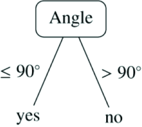
A good approximate model for predicting whether or not the robot will move closer to a non-moving object (i.e., object A or B) after performing one of its actions. Note that in this tree, the prediction does not depend on Action and Distance.

Suppose the robot performed three actions: “left”, “left” and “right”, as shown in Fig. 2. While performing these actions, it collected nine learning examples, three for each object, as given in Table 1. At this point the robot stopped and built a decision tree for each object. Since the robot is not able to build a highly accurate model for a quickly moving object (i.e., object C), we will focus our attention on prediction models for objects A and B. They are shown in Fig. 4(a) and Fig. 4(b), respectively. The decision tree built on the examples corresponding to object A is similar to the good approximate model presented in Fig. 3. The only difference is its inaccurate Angle split point (59° instead of 90°). On the other hand, the decision tree built on the examples for object B is quite different from the good approximate model, since it only contains one leaf, which classifies all the examples as MovedCloser = “yes”.

Figure 4.

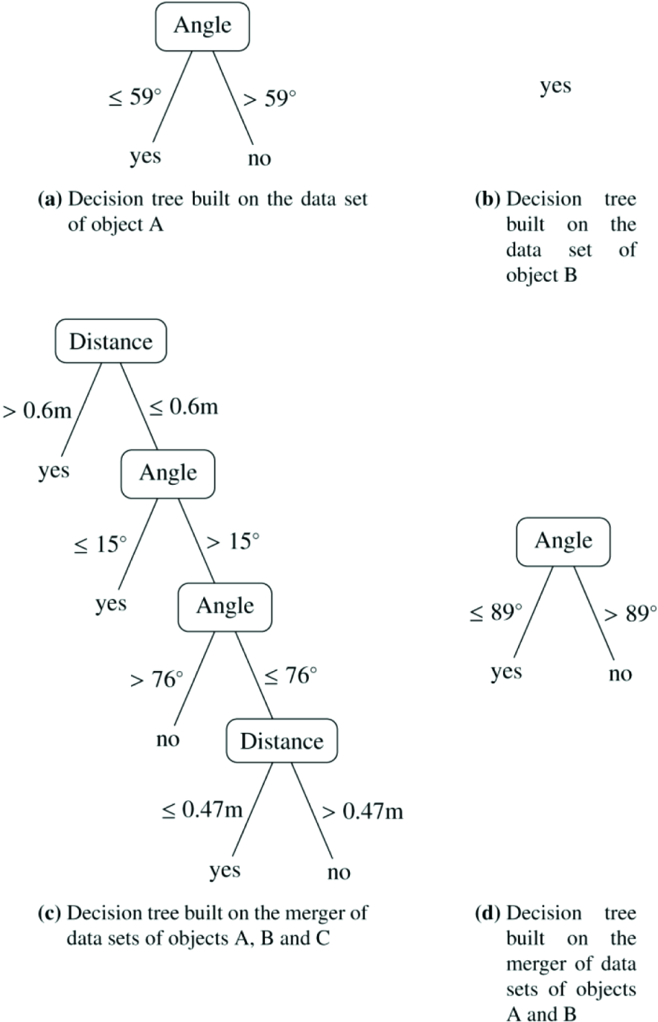
Decision trees built by the robot corresponding to different learning data sets. The leaves indicate the value (either “yes” or “no”) of class MovedCloser.

Table 1.

Data table with nine learning examples, three for each object, that the robot collected while performing the three actions shown in Fig. 2

	Distance	Angle	Action	MovedCloser
object A	0.37m	10°	left	yes
	0.17m	108°	left	no
	0.46m	179°	right	no
object B	1.01m	21°	left	yes
	0.67m	12°	left	yes
	0.42m	70°	right	yes
object C	0.52m	20°	left	no
	0.81m	120°	left	yes
	0.53m	82°	right	no

With the aspiration of building a more accurate model for object A or B, the robot may try to merge (i.e., concatenate) the data sets of individual objects. In this way it will obtain data sets with more learning examples, which may lead to building more accurate prediction models. If the robot naïvely merges all examples of all objects and builds a decision tree, it will get the tree shown in Fig. 4(c). This tree is very far from the desired prediction model shown in Fig. 3. It is actually a lot worse than the trees built on each individual learning set of objects A and B. However, if the robot only merges the data sets corresponding to objects A and B, it gets a very good prediction model shown in Fig. 4(d). This tree is identical to the good approximate model in Fig. 3, except for the negligible difference (1°) in the Angle split point. With this simple example we have shown how the robot might build a more accurate model by merging data sets of objects of the same type. It should be noted, again, that the robot does not know the types of objects. So the question of what data to merge advantageously is a difficult challenge. In the above example, we have also demonstrated how naïve merging of all data can lead to undesirable results.

In this paper we present a new learning algorithm which exploits the greater complexity of an environment with more objects to speed up the learning of a model for a single object. The speed-up is achieved through intelligent merging of traces of observations for different objects that assumingly behave in the same way (an object's trace contains the sensors' measurements for this object). By increasing the number of learning examples, a machine learning algorithm can build a more accurate model. The merging of objects' traces is accomplished by observing the average prediction errors of models built on separate and merged objects' traces, and following a set of criteria that determine whether or not the merging of traces would be beneficial.

The rest of the paper is organized as follows. First, in section 2, we briefly review the related work. In section 3 we give a detailed description of our experimental domain and present the relation the robot tries to learn, namely how the robot's distance to an object changes after it performs one of its actions. We also define the terms cardinal complexity, behavioural complexity and behaviour class, and present a series of scenarios which define increasingly more complex worlds, in which the robot tries to learn the aforementioned relation. Next, in section 4, we present Error reduction merging (ERM), our proposed learning algorithm. We start by presenting the main ideas and giving a general overview of the algorithm, and in later subsections we describe the details of the algorithm along with its pseudo-code. Section 5 describes the experimental setup we used to evaluate the performance of our proposed ERM learning method. The experimental results along with comments and discussion are presented in section 6. Lastly, in section 7, we present our conclusions and give some possibilities for future work in this area.

2. Related work

Our investigation of how the complexity of the environment (in terms of the number of objects and their distinct behaviours) may offer the possibility of speeding up an agent's learning process is, to our knowledge, the first such study. The following subsections present some existing work, which is in certain aspects similar to ours. We give a brief description of the work and explain which of the ideas presented are related to our research.

2.1. Transfer learning

A very interesting research area that is related to our work is transfer learning [2]. In particular, our setting is most similar to inductive transfer learning, where labelled data is available for both the target and the source domain. In our setting, the target domain would correspond to the domain of the object for which the robot is learning a prediction model. The source domains would be the domains of all other objects. Inductive transfer learning methods try to identify which parts of the source data are “good” and which parts are “bad” for transferring to the target domain. This is similar to how our ERM learning method has to discern which objects to merge with the current target object to speed up the learning of the prediction model for the target object. Examples of such transfer learning techniques are TrAdaBoost [3] and M-Logit [4].

2.2. Cooperative multi-agent learning

Another research area that is also related to our exploration of achieving learning speed-ups by learning in a more complex environment is cooperative multi-agent learning [5]. Our problem setting, where an agent simultaneously observes multiple objects and exploits this as a kind of parallel data collection, is in a way analogous to the problem setting with multiple agents where each agent observes one object and the agents learn cooperatively by sharing the collected data between each other.

A learning approach where two robots learn simultaneously and share their experiences is presented in [6]. The task of the robot is to learn reactive behaviours for avoiding obstacles. On each time step the robot transmits the following information to the other robot (and vice versa): the position of the object it reacted to, the action it chose and how good it was. Effectively, this means that the two robots act as one learning agent with twice as much learning data, which is in a way similar to our ERM learning method, which also increases the amount of learning data by using data from observations of other similar objects. They have shown that this sharing of experiences results in a faster and more repeatable learning of the robot's behaviours. Their work assumes that the target models are the same for both robots. In our work, however, the learner has to find out whether such assumptions are justified.

A study of how to automatically design multi-agent systems of cooperative agents, where each agent learns independently, was performed by [7]. They used an incremental learning scheme, where they progressively increased task complexity and multi-agent system complexity. The idea behind the approach is that agents are able to re-use a learned policy in a more complex environment, which leads to faster learning. Simultaneously with increasing the number of learning agents, they also added other objects to the environment, which also increased the complexity of learning. Although in our case we only observed one agent learning a single classifier, the idea of increasing the complexity of the environment by increasing the number of different objects is similar to ours.

2.3. Speeding up reinforcement learning

Many reinforcement learning (RL) [8] techniques, which try to decrease the amount of time steps before converging towards a good policy, have been proposed. We will describe a few examples which bear some similarities to our approach.

A study of how RL can be used to “shape” a robot to perform animal-like behaviours (e.g., chasing prey, escaping from predators, etc.) was performed in [9]. The part of the paper that touches on the issue of learning speed is the design of an agent's architecture. They demonstrated that by carefully designing an agent's architecture by decomposing a complex behaviour pattern into simpler ones, the learning can be accelerated as a result of the narrowed search. This is in some way related to our object-oriented decomposition of the robot's learning data, which ERM can exploit to find similarly behaving objects.

An algorithm for efficient structured learning in factoredstate Markov Decision Processes (MDPs) was proposed in [10]. A factored-state MDP is one whose states are represented as a vector of distinct features, which is similar to our representation of the experimental domain. Their approach seeks to maximize experience, which would be, in our terms, analogous to maximizing the amount of learning examples. This is akin to what ERM strives for—maximizing the number of learning examples with the aspiration of building more accurate prediction models.

An interesting approach is the use of object-oriented representation for more efficient RL presented in [11]. Therein they proposed object-oriented MDPs, an extension to the standard MDP formalism which is based on attributes that can be directly perceived by the agent. This representation is similar to our object-oriented representation of the experimental domain. They have shown that this representation scales very well with respect to the size of the state space, which makes RL feasible in larger state spaces. Since our learning task is limited to building a model for each object independently of other objects, our learning method does not have to cope with such scaling problems.

2.4. Learning by experimentation

Our learning task is a case of learning by experimentation. The foundations of learning by experimentation lie in the field of computational scientific discovery [12]. Early work includes the BACON discovery system developed by Langley [13, 14, 15], which is capable of rediscovering a number physical laws from collected empirical data. An overview of the history of computational scientific discovery is given by Darden [16] and Langley [17].

The experimental domain and the learning task that we used for our experiments follows a similar setting as [18]. They used an autonomous learning robot that built qualitative models for predicting how the robot's distance and angle to an object change after it performs one of its actions.

3. Experimental domain

Our problem domain consists of an autonomous mobile robot, objects of different types and an overhead camera. The robot uses the overhead camera to observe its distance to each of the objects (denoted by dist) and the angle between its orientation and each of the objects (denoted by ang), as shown in Fig. 5. For calculating distances and angles, all the objects are approximated with points—their centres of gravity.

Figure 5.

Robot uses the overhead camera to observe its distance to each of the objects (dist) and the angle between its orientation and each of the objects (ang).

At each time step the robot executes one of the following actions (denoted by action): move straight ahead, move left or move right, as shown in Fig. 6. The robot avoids actions that lead to collision.

Figure 6.

Robot's actions: move straight ahead, move left and move right. At each time step the robot executes one of these actions.

The robot has no built-in concept of a coordinate system. All it knows are its actions and observations about surrounding objects. An example of a data trace that the robot collects during its learning process is given in Table 2. The value of an attribute a at time step t will be denoted by a^t

Table 2.

An example of a data trace that the robot collects during its learning process

Time	object 1		…		object k	…
Step	dist ₁	ang ₁	…	dist_k	ang_k	…	action
1	0.5m	30°	…	0.4m	10°	…	left
2	0.7m	50°	…	0.1m	-10°	…	right
3	0.4m	80°	…	0.3m	20°	…	right
⋮	⋮	⋮		⋮	⋮		⋮

The robot is aware of the fact that it observes the same set of attributes for each object and which measurements belong to which object. For example, the robot knows that attributes dist_k and dist_l both measure the same thing (robot's distance to an object), the first with respect to object k and the second with respect to object l.

3.1. Learning the change in object distance

The robot's goal is to build a model for predicting the change in its distance to an object after executing one of its actions. Rather than predicting the exact value of the change, we want the robot to build a qualitative model for predicting the qualitative change in its distance to an object. This can either be increased (+) or decreased (-) (theoretically, there is also a third possibility: no change (o), however, it occurs so rarely that we merged it with +).

More precisely, for object k, the robot will build a model M_k for predicting the change in distance between the robot and the object in the next time step (sgn(Δdist^t_k^{+ 1})) after executing an action (action^t) in the current state (dist^t_k, ang^t_k):

sgn (Δ d i s t_{k}^{t + 1}) = M_{k} (d i s t_{k}^{t}, a n g_{k}^{t}, a c t i o n^{t}),

where Δdist_k^t⁺¹ = dis^t⁺¹_k - dist^t_k.

To simplify the learning of model M_k, the robot will assume the model is a function of attributes pertaining to the particular object (i.e., dist_k and ang_k) and robot's action (action) only.

A simple approximate model of the qualitative change in the robot's distance to an object k can be summarized using the following three rules:

(1)

IF ang< - 90° THEN

sgn(Δdist_k^t+¹) = +,

(2)

IF - 90° ≤ ang ≤ 90° THEN

sgn(Δ dist_k^t+¹) = -,

(3)

IF ang>90° THEN

sgn(Δ dist_k^t+¹) = +.

A graphical illustration of these rules is given in Fig. 7. In section 5, we present the accuracy of these rules on an independent testing set along with a discussion of the misclassified examples.

Figure 7.

A graphical illustration of the rules for the qualitative change in robot's distance to an object. The figure pictures a case when the robot starts at ang = 0° and moves either left or right.

In this paper, we are interested in minimizing the number of examples needed for learning (i.e., how many examples are needed to achieve a certain prediction accuracy). This is a common criterion in machine learning. In our experimental domain with a robot collecting learning data, this corresponds to the time needed for successful learning (i.e., how many actions are needed to achieve a certain prediction accuracy). Since minimizing the total experimentation time by a robot is often a reasonable and appropriate optimization criterion, we also chose it for our experiments.

We are aware of the fact that this is a very simple robotic domain. Nonetheless, we think it is rich enough for performing a set of interesting experiments. At the same time, we feel that precisely its simplicity offers us a clear way of evaluating our ideas and answering the questions we set at the beginning of this paper.

3.2. Scenarios with worlds of increasing cardinal and behavioural complexity

The robot's learning process will take place in different worlds of increasing cardinal and behavioural complexity. We define the cardinal complexity as the number of objects in the robot's world. The greater the number of objects in the robot's world is, the greater is its cardinal complexity. Similarly, we define the behavioural complexity as the number of objects' behaviour classes. A behaviour class is a set of objects that behave in the same way with respect to the particular relation the robot is modelling (i.e., change in object's distance). The more behaviour classes there are in the robot's world, the greater is its behavioural complexity.

We will use objects from two behaviour classes: static (non-moving) objects and moving objects. The robot will only be able to model the change in its distance to an object from the first class, since, in this case, the change depends on the previous state of the object (dist^t, ang^t) and the robot's last action (action^t). Objects from the second class will move randomly, thereby preventing the robot building a highly accurate model for predicting the change in its distance to such objects. We chose boxes as representatives of the static class and mobile robots as representatives of the moving class.

To obtain worlds of increasing cardinal and behavioural complexity, we constructed the following scenarios:

1 box (1B),

2 boxes (2B),

4 boxes (4B),

4 boxes and 4 mobile robots (4B4R),

4 boxes and 8 mobile robots (4B8R).

Every scenario also includes an autonomous mobile robot which observes the world and learns. Initially, the autonomous mobile robot, boxes and other mobile robots are randomly placed in a rectangular playground enclosed with a wall on each side. Three examples of such scenarios are pictured in Fig. 8.

Figure 8.

Three examples of scenarios showing worlds of increasing cardinal and behavioural complexity.

The robot's goal is the same in all scenarios: learn a model for predicting the sgn(Δdist^t+¹) for each object in a given scenario. By using different scenarios, we will try to answer some interesting questions: “Is it possible to speed up the learning of the model for one box when we have information about another box?” “What about when we have information about three more boxes?” “How does the presence of objects from a different behaviour class affect the speed of learning?” “Will the proposed method be able to recognize which objects belong to the same behaviour class?” “How does the method cope when we further increase the number of objects belonging to the different behaviour class?”

4. Error reduction merging (ERM)

4.1. Merging objects' data

When the robot is concurrently learning a model for predicting the change in its distance to an object k, it collects a trace of examples of the form (dist^t_k, ang^t_k, action^t), one example at each time step t. To convert this trace to a learning set, it computes the sgn (Δdist_kt⁺¹) for each pair of consecutive examples in the trace.

Moreover, it collects such traces and converts them to learning sets for all the objects it observes through the overhead camera. If it knew which objects belong to the same behaviour class with respect to the change in object's distance (as described in section 3.2), it could extend the learning set of this particular object k with the learning sets of all other objects from the same behaviour class. This way, it would considerably multiply the number of learning examples used to build this model. Since other objects are located in distinct parts of the robot's playground, we expect their learning sets to at least partially differ from the learning set of the chosen object. Furthermore, if objects are indeed from the same behaviour class, then their learning sets will complement the learning set of the chosen object in examples covering distinct parts of the attribute space. Also, their learning sets will not conflict with the learning set of the chosen object in examples covering the same parts of the attribute space. Hence, we can expect the accuracy of the induced model to increase.

However, since the robot does not have information about which objects belong to the same behaviour class, it can only hypothesize about that at each time step. Its hypotheses are based on models built on the current learning sets of the objects.

Let $l_{o_{i}}$ and $l_{o_{j}}$ represent the learning sets of objects o_i and o_j, respectively. Merging learning sets $l_{o_{i}}$ and $l_{o_{j}}$ means the following: first, the corresponding attributes of both objects are unified (e.g., dist_i and dist_j are treated as the same attribute), and then the corresponding data series are concatenated. Let $l_{o_{i}} + l_{o_{j}}$ denote the merger of learning sets $l_{o_{i}}$ and $l_{o_{j}} .$ .

When determining whether merging objects objects o_i and o_j (i.e., their learning sets) would be beneficial, the algorithm builds three models with the same base learner, one on $l_{o_{i}},$ , one on $l_{o_{j}}$ and one on $l_{o_{i}} + l_{o_{j}},$ , and compares them on selected combinations of the learning data sets $(l_{o_{i}}, l_{o_{j}}, l_{o_{i}} + l_{o_{j}}) .$ .

Let Ē(o_r, o_s) denote the average prediction error of a model built on the learning set of object o_r and tested on the learning set of object o_s. Ē(o_r, o_s) here means a particular error estimate, a kind of generalized leave-one-out cross-validation method which will be explained in detail in section 4.2. We can now define the error reduction (ER) of merging objects o_i and o_j as follows:

E R_{o_{i}, o_{j}} = \frac{{| l}_{o_{i}} | \bar{E} (o_{i}, o_{i}) + {| l}_{o_{j}} | \bar{E} (o_{j}, o_{j})}{{| l}_{o_{i}} | + {| l}_{o_{j}} |} - \bar{E} (o_{i} + o_{j}, o_{i} + o_{j}) .

(1)

A positive ER indicates that the weighted average of average prediction errors of models built and tested on each object's learning set is greater than the average prediction error of a model built and tested on the merger of objects' learning sets. This implies that by merging objects o_i and o_j the average prediction error on their respective learning sets would be reduced. This will become our main criterion for deciding whether or not the learning algorithm should merge two objects.

After the robot has performed a certain number of actions, it stops and runs the merging algorithm on the newly augmented objects' traces. First it converts the traces to learning sets (as described before) and then it starts to evaluate which objects to merge at the current iteration. It merges objects agglomeratively, similarly to hierarchical clustering [19], starting with the two objects that are the best candidates for merging and continuing until either there is only one (merged) object left or the remaining object pairs do not pass the criteria for merging.

A pair of objects (o_i, o_j) is a candidate for merging if it passes the following criteria:

(1)

both learning sets, $l_{o_{i}}$ and $l_{o_{j}},$ , contain a minimal number of examples (controlled by parameter n),

(2)

the ER of merging objects o_i and o_j is greater or equal to zero.

The first criterion is a rudimentary threshold that eliminates all candidate pairs whose learning sets are too small. When the learning set of an object is very small, it makes little sense to try to ascertain whether or not this object belongs to the same behaviour class as some other object.

The second criterion compares the average prediction errors of all three models (built on $l_{o_{i}}, l_{o_{j}}$ and $l_{o_{i}} + l_{o_{j}})$ on their own data sets. As dictated by Eq. (1), the average prediction error of a model built and tested on the merged data set has to be lower or equal to the weighted average of the average prediction errors of the individual models on their respective learning sets. This criterion will ensure that by merging objects o_i and o_j the average prediction error on their respective learning sets will not increase.

However, solely observing the size of ER is not the best way to choose the next pair of objects to be merged, as can be illustrated with a simple example. Suppose that learning instances are points lying on a one-dimensional line, and the class function is a simple binary thresholding function f parameterised by θ:

f (x) = {\begin{array}{l} + & if x > θ, and \\ - & otherwise . \end{array}

Furthermore, suppose we have a candidate pair of objects (o_i, o_j) with learning sets as pictured in Fig. 9. By using a machine learning algorithm on all combinations of these learning sets $(l_{o_{i}}, l_{o_{j}}$ and $l_{o_{i}} + l_{o_{j}}$ ), we obtained three models giving different approximations of θ : $θ_{o_{i}}, θ_{o_{j}}$ and $θ_{o_{i} + o_{j}}$ (also pictured in Fig. 9). The average prediction errors of these models on their learning sets are all equal to zero. Hence, ER is zero. Our merging criterion (2) is therefore satisfied, but the gain from merging is zero. In comparison with other candidate pairs of objects, the pair (o_i, o_j), according to ER, does not look very attractive. However, observing the learning examples of o_i and o_j, it would be natural to merge these two objects together, as their learning sets complement one another very well. When merged, these examples determine θ very accurately. This example shows that ER may underestimate the benefit of merging a pair of objects. Therefore ER is not a good criterion for ranking candidate pairs of objects to be merged.

Figure 9.

A simple example illustrating the shortcoming of solely observing ER. Learning instances are points lying on a one-dimensional line, and their class values are either + (if x > θ) or - (otherwise). The upper and lower parts represent the learning sets of objects o_i and o_j, respectively, each one containing five learning examples. By using a machine learning algorithm on all combinations of these learning sets $(l_{o_{i}}, l_{o_{j}}$ and $l_{o_{i}} + l_{o_{j}}$ ), we obtained three models giving different approximations of

A solution to this issue is to check whether the following inequalities hold:

\bar{E} (o_{i} + o_{j}, o_{i} + o_{j}) \leq \bar{E} (o_{i}, o_{i} + o_{j}),

(2)

\bar{E} (o_{i} + o_{j}, o_{i} + o_{j}) \leq \bar{E} (o_{j}, o_{i} + o_{j}) .

(3)

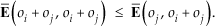
If the learning sets of objects o_i and o_j complement one another well in examples covering distinct parts of the attribute space, these inequalities will hold. In addition, criterion (2) (i.e., ER ≥ 0) ensures that the learning sets of these two objects do not conflict with each other in examples covering the same part of the attribute space.

Returning to the previous example, the remaining average prediction errors are the following:

\begin{array}{l} \bar{E} (o_{i}, o_{i} + o_{j}) = 3 / 10, \\ \bar{E} (o_{j}, o_{i} + o_{j}) = 2 / 10 . \end{array}

Clearly, both inequalities from Eq. (2) and (3) hold, which is in accordance with the intuition that it would be beneficial to merge objects o_i and o_j.

To rank the candidate pairs of objects, we observe to what extent the pairs' learning sets cover the same part of the attribute space, and to what extent the pairs' learning sets cover distinct parts of the attribute space. We want to merge the pair of objects that cover as much of the attribute space as possible in order to build a good model for the whole attribute space.

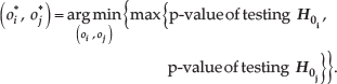
Ranking of candidate pairs of objects is achieved by performing a series of t-tests comparing the average prediction error of each object's model with the average prediction error of the merged object's model. For each candidate pair of objects (o_i, o_j) two one-sided t-tests testing the following null hypotheses:

H_{0_{i}} : \bar{E} (o_{i}, o_{i} + o_{j}) \leq \bar{E} (o_{i} + o_{j}, o_{i} + o_{j}),

(4)

H_{0_{j}} : \bar{E} (o_{j}, o_{i} + o_{j}) \leq \bar{E} (o_{i} + o_{j}, o_{i} + o_{j}),

(5)

are performed. A higher p-value signifies a weaker rejection of a null hypothesis. We want to reject both null hypotheses, $H_{0_{i}}$ and $H_{0_{j}},$ , with as much statistical significance as possible, so we choose the best candidate pair of objects (o*_i, o*_j) to be the one with the minimal maximal p-value:

\begin{array}{l} (o_{i}^{*}, o_{j}^{*}) = \underset{(o_{i}^{}, o_{j}^{})}{arg min} {max {p-value of testing H_{0_{i}}, \\ p-value of testing H_{0_{j}}}} . \end{array}

After merging objects o*_i and o*_j into o_m, all possible pairs of objects containing o_m are generated and tested against the criteria (1) and (2). In addition, the algorithm checks if they satisfy the inequalities from Eq. (2) and (3). The pairs of objects that pass the criteria and satisfy the inequalities are added to the set of candidate pairs and the ranking process is repeated. This is continued until there are no more candidate pairs left (details of the merging procedure are explained in section 4.3).

When the merging at current iteration is finished, the models for the remaining (merged) objects are built and tested on the independent testing set (as will be described in section 5). Afterwards, the objects are split again and the robot continues executing new actions and augmenting the objects' traces. After a certain number of actions (controlled by the parameter u described in section 4.4), it stops and runs the same merging algorithm from the beginning.

The following three subsections give a detailed description of the presented learning algorithm. Each subsection also contains the pseudo-code of a part of the algorithm. In section 4.2, we present the ESTIMATE-ERRORS-AND-SIGNIFICANCES procedure, which uses the GENERALIZED-LEAVE-ONE-OUT procedure to estimate the average prediction errors of different models on selected combinations of the learning sets. In addition, ESTIMATE-ERRORS-AND-SIGNIFICANCES performs two pair-wise one-sided t-tests testing the null hypotheses H _0i and H _0j presented earlier. Next, in section 4.3, we present the ERM method which forms the central part of the robot's learning algorithm. Finally, in section 4.4, we describe the LEARNING-LOOP procedure which is the high-level learning algorithm running on our autonomous robot.

4.2. Estimating the average prediction errors and significances using a generalized leave-one-out method

Let us define the prediction error of a model M for an example x as:

e_{M} (x) = 1 - {\overset{⌢}{P}}_{M} (y^{*} | x),

where ${\overset{⌢}{P}}_{M} (y | x)$ is the model's predicted probability of example x having class value y, and y* denotes the example's true class value.

To estimate the average prediction errors of different models (obtained by training the same base learner on different learning sets) on selected combinations of the learning sets, we used the ESTIMATE-ERRORS-AND-SIGNIFICANCES procedure as given in Fig. 10. In addition, this procedure also performs two pair-wise one-sided t-tests testing the null hypotheses $H_{0_{i}}$ and $H_{0_{j}}$ described in section 4.1. We use P (o_r, o_s; o_t) to denote the p-value of a pair-wise one-sided t-test testing the null hypothesis: Ē(o_r, o_t) ≤ &Emacr;(o_s, o_t).

Figure 10.

The ESTIMATE-ERRORS-AND-SIGNIFICANCES procedure estimates the average prediction errors of different models on selected combinations of the learning sets and computes the p-values of two one sided t-tests testing the null hypotheses from Eq. (4) and (5). The GENERALIZED-LEAVE-ONE-OUT procedure is a generalized leave-one-out cross-validation method that estimates the average prediction error of models built on the learn set and tested on examples from the test set. It should be noted that the purpose of the above procedure is to define what the result of generalized leave-one-out is, and not that it should actually be implemented in this inefficient way.

The input to the ESTIMATE-ERRORS-AND-SIGNIFICANCES procedure are a machine learning algorithm A that is used to build the models, and objects o_i and o_j that are candidates for merging at the current iteration. Algorithm A is assumed to produce models that, for a given example, return probability distribution over all class values.

The output of the ESTIMATE-ERRORS-AND-SIGNIFICANCES procedure is a pair (&Emacr;, P), where &Emacr; is the set of computed average prediction errors Ē(., .), and P is a set of p-values of the computed t-test statistics P(., .;).

The main part of the ESTIMATE-ERRORS-AND-SIGNIFICANCES procedure (lines 2-6) are calls to the GENERALIZED-LEAVE-ONE-OUT procedure that computes the average prediction errors of selected combinations of the learning sets. In the last part (lines 7–8), Estimate-errors-and-significances performs two pair-wise one-sided t-tests testing the null hypotheses $H_{0_{i}}$ and $H_{0_{j}}$ as defined in Eq. (4) and (5).

The average prediction error of a model built on a given learning set and tested on examples from a given testing set is computed with the Generalized-leave-one-out procedure which performs a kind of generalized leave-one-out cross-validation to avoid biased prediction error estimates. The pseudo-code of the Generalized-leave-one-out procedure is also given in Fig. 10.

The input to the Generalized-leave-one-out procedure are a machine learning algorithm A that is used to build the models and two data sets: learn, which contains the learning examples, and test, which contains the testing examples.

The output of the Generalized-leave-one-out procedure is the average prediction error of models built on the learn set and tested on examples from the test set.

The procedure iterates through the for loop and estimates the prediction error of each example x from the test set. It creates a model M built on the whole learn set, excluding the current testing example x if it is also contained in the learn set (line 2). Then it computes the prediction error of M for the current testing example (line 3).

The difference with the standard leave-one-out [19] is that Generalized-leave-one-out takes two data sets as input. The first one is the learning set which is used to build the model and the second one is the testing set which is used to test the model. On each iteration the algorithm checks if the currently tested example is in the learning set. If yes then this example is not used for learning in this iteration. This gives us better error estimates since the tested example is never included in the learning set that was used to build the model. We can also observe two special cases of using the Generalized-leave-one-out procedure: if the learning and testing set are the same, it performs the standard leave-one-out. If the learning and testing set have no examples in common, it performs the standard testing procedure with two disjoint data sets, one for learning and the other for testing.

4.3. Merging objects using the ERM method

The central part of the robot's learning algorithm is the ERM learning method presented in Fig. 11.

Figure 11.

The pseudo-code of the Error reduction merging (ERM) method, which forms the central part of the robot's learning algorithm.

The input to the ERM method are the set of current objects O, the set of current objects' learning sets L, parameter n controlling the minimal number of examples in a learning set, and a machine learning algorithm A that is used to build the models inside the calls to the ESTIMATE-ERRORS-AND-SIGNIFICANCES procedure.

The output of the ERM method is a triplet (O, L, M), where O represents the new set of objects, L represents the new set of objects' learning sets (after merging) and ℳ represents the set of models built on the new objects' learning sets.

First (line 1), the method initializes set C that will hold object pairs that are candidates for merging. The following for loop (lines 2-8) iterates through all object pairs (o_i, o_j) ϵ O and adds them to the set C if they pass the following criteria:

(1)

both learning sets, $l_{o_{i}}$ and $l_{o_{j}}$ , contain at least n examples,

(2)

the ER of merging objects o_i and o_j is greater or equal to zero,

(3)

the average prediction error Ē(o_i+o_j, o_i+o_j) satisfies the inequalities from Eq. (2) and (3), that is:

Ē(o_i +o_j, o_i +o_j) ≤ min {&Emacr;(o_i, o_i +o_j), Ē(o_j, o_i +o_j)}.

Explanation of these criteria was given in section 4.1.

After filling the set C with candidate pairs that pass these criteria, the method iterates through the while loop (lines 9-23), as long as there are still candidates pairs left to be merged. The chosen pair (o*_i, o_j*) on each iteration is the one with minimal maximal p-value of the t-test statistics obtained by testing the null hypotheses $H_{0_{i}}$ and $H_{0_{j}}$ as defined in Eq. (4) and (5) (line 10).

After creating a new object and merging the learning sets of the chosen objects (lines 12-13), the method updates O by removing the chosen pair of objects and adding the newly created object (line 14) and L by removing the learning sets of the chosen pair of objects and adding the learning set of the new object (line 15). In addition, all candidate pairs that contained either o*_i or o*_j are removed from C (line 16).

The nested for loop (lines 17-23) works the same way as the first for loop (lines 2-8), except that it now fills C with candidate pairs that contain the newly created object o_m.

Finally, the method initializes set ℳ that will hold the models built on the new objects' learning sets (line 24). The following for loop (lines 25-28) iterates through all (merged) objects from the final set O. It builds a model on each object's learning set and adds it to the set ℳ

4.4. Learning algorithm running on the robot

The high-level learning algorithm running on our autonomous robot takes the form of a simple learning loop, as presented in Fig. 12.

Figure 12.

High-level learning algorithm running on our autonomous robot.

The parameters given to the LEARNING-LOOP procedure are the interval (i.e., the number of time steps) between two successive calls to the ERM method denoted by u, the minimal number of examples in a learning set denoted by n, and a machine learning algorithm A that is used to build the models inside the calls to the ERM method.

After initializing sets $O, T, L$ (lines 1-3) and iteration counter t (line 4), the LEARNING-LOOP starts executing its main loop. At each time step t, the robot receives information about its distance to each of the objects ({dist^t_o1, dist^t_o₂,…, ({ $d i s t_{o_{1}}^{t}, d i s t_{o_{2}}^{t}, …, d i s t_{o_{| O |}}^{t}$ }) and the angle between its orientation and each of the objects ({ $a n g_{o_{1}}^{t}, a n g_{o_{2}}^{t}, …, a n g_{o_{| O |}}^{t}$ }) and updates objects' current traces and learning sets (lines 7-8).

When $t \equiv 0 (\mod u)$ , the algorithm first backs up the current sets O and L (line 10) and then proceeds with the call to the ERM method (line 11). After obtaining the ERM's results, it restores sets O and L to their values from before the merging (line 12). This will cause the merging to start from the beginning on the next call to the ERM method.

At the end of the loop, the algorithm chooses one of the possible actions (as described in section 3) and executes it (line 13).

5. Experimental setup

We implemented our experiments in the Webots robot simulator [20]. The autonomous learning robot and other mobile robots were implemented as simple differential wheeled robots. At every time step, each robot randomly chose one of the possible actions (as described in section 3) and executed it. Technically, collision avoidance was implemented as follows: all of the robots had a front bumper which served as a touch sensor. Whenever a robot's touch sensor detected a collision, the robot stopped executing its current action and performed a simple avoidance manoeuvre: it moved back and turned a bit to the left. Then it continued executing its actions. Every action the robot commenced executing counted as one iteration of the learning algorithm.

In order to represent objects from a different behaviour class with respect to the relation the robot is learning, the other mobile robots had to move substantially faster than the autonomous learning robot. If they had moved as fast as the learning robot, they would have been indistinguishable from the static boxes, since the robot is only modelling the qualitative change (i.e., the sign of the change) in its distance to an object.

The vision system with the overhead camera was simulated with a special Webots controller named supervisor, which had access to all the information about the learning robot and other objects currently simulated. At every time step, the supervisor read the positions and orientations of the learning robot, and other objects. It then computed the learning robot's distance to each of the objects (dist), and the angle between its orientation and each of the objects (ang). Finally, this information was packed in a message and sent to the learning robot. Note that the learning robot never had information about the objects' coordinates, but only about each object's dist and ang values as computed by the supervisor.

The rectangular playground in which the learning robot and other objects were enclosed was of size 2.0 m × 2.0 m. The boxes were implemented as cubes with sides of length 0.1 m. All the robots were of the same shape and size, and their size was approximately the same as the size of a box.

We used three distinct base machine learning methods inside our ERM and other learning methods (described later in this section), namely naïve Bayes classifier (NBC) [19], C4.5 decision tree learner [1] and support vector machines (SVM) [21]. The particular implementation of these methods was the one provided in the Orange machine learning and data mining suite [22].

The NBC used locally weighted regression (LOESS) [23] with parameter window_proportion = 0.1 (proportion of examples used for local learning in LOESS) for the estimation of (conditional) probabilities of continuous attributes. Other parameters were left at their default values.

For the C4.5 learning algorithm we used the default parameter settings.

The parameters of the SVM were: svm_type = C-SVC (type of the SVM formulation), C = 100 (regularization parameter), kernel_type = polynomial (type of the kernel function), degree = 3 (degree of the polynomial kernel), coef_0 = 1 (value of the constant term of the polynomial kernel). Other parameters were left at their default values.

For practical reasons, we chose to only use NBC throughout the first two sets of experiments. At the end we give a comparison of all three base machine learning methods on our most complex scenario (as defined in section 3.2).

To assess the performance of our ERM learning method, we took the set of models ℳ, tested each model on an independent testing set (described later) and recorded its classification accuracy (CA). Since the robot was not able to build a highly accurate model for predicting the change in its distance to objects from the moving behaviour class (i.e., mobile robots), we were only interested in classification accuracies of models for the objects from the static behaviour class (i.e., boxes). We took the average CA of all models containing predictions for boxes as the final CA (e.g., when the ERM method erroneously merged a box with mobile robots, we also took that model into account since the robot would use this model when asked to predict the change in its distance to this box). This testing was done after every call to the ERM method (line 11 of the LEARNING-LOOP presented in Fig. 12).

In our experiments, we chose to run ERM each time after the next five actions were completed (i.e., we set parameter u to five). A comment is in order regarding the rate of model updates during a learning run. In this paper, we are interested in studying the dependence between the number of actions and the corresponding prediction accuracy achieved by ERM vs. other merging strategies (described later). In a practical application of ERM, the user may choose to update the prediction model obtained by ERM at different rates. In particular, for best accuracy at any time during learning, ERM would be executed after each action. In the case of a relatively fast acquisition of new data, the process of model updating could possibly lag behind the data acquisition process. In this case, it would be reasonable to restart the model update immediately after the previous model update was completed. Another idea would be to find a metric that would indicate whether a model update is warranted. The observed critical value of this metric would warrant a next model update.

The parameter n, controlling the minimal number of examples in a learning set before it is considered for merging, was set to five.

To evaluate the learned models, we generated a separate testing set. This set was obtained by densely sampling the attribute space with one object and observing the real change in the robot's distance to the object after executing an action. We created a grid sample with 10 initial x coordinates of the robot, 10 initial y coordinates of the robot, 12 initial robot's orientations and three actions that the robot performed from the initial position. The object that the robot observed was a box placed in the centre of the playground. This way we obtained 3600 examples against which we tested our models to measure their CA.

Note that our simple approximate model of the qualitative change in the robot's distance to an object (presented in section 3.1) is only 91.75% accurate on this testing set. By observing the misclassified examples, we discovered some common patterns. All misclassified examples have ang on interval (70°, 100°) or (−100°, −70°). There are two major types of misclassified examples:

Examples that have ang ϵ (70°, 90°) and action = left and examples that have ang ϵ (−90°, − 70°) and action = right. In both cases, executing an action results in an increase of the robot's distance to an object (+), contrary to what rule (2) would have predicted (-). They represent 51% of misclassified examples.

Examples that have ang ϵ (90°, 100°) and action = right and examples that have ang ϵ (−100°, −90°) and action = left. In both cases, executing an action results in a decrease of the robot's distance to an object (-), contrary to what rules (1) and (3) would have predicted (+). They represent 19% of misclassified examples.

Other misclassified examples do not exhibit a common pattern.

For quantifying the relative performance of our ERM learning method, we compared it with the following three merging strategies:

NoMerging: No objects are merged with this strategy. The learning algorithm only uses the data of each object to build its particular model. This “merging” strategy will serve us as a baseline when evaluating the learning performance of our ERM method.

Oracle: With this strategy, we assume we have an oracle that tells the learning algorithm, which objects belong to the same behaviour class, so it can merge them on the first learning iteration. This merging strategy will serve us as the upper bound for the learning performance of our ERM method.

MergeAll: This merging strategy merges all objects at the first learning iteration, regardless of whether or not they belong to the same behaviour class. As such it will serve us as another baseline when evaluating the learning performance of our ERM method.

We constructed a learning curve for each merging strategy depicting how the strategy's CA increases with the number of iterations. To obtain a learning curve, we repeated the same experiment 100 times, each time with different randomly chosen initial positions and orientations of the learning robot and the other objects. Each learning curve represents the mean of 100 repetitions of the experiment. Errors bars show 95% confidence intervals for the means.

6. Experimental results

The following results try to answer the questions raised at the end of section 3.2. They are divided into three parts, each dealing with a certain aspect of the experimental domain. The first part covers the increase in the world's cardinal complexity due to an increasing number of boxes present in the world. The next part investigates the scenarios with a constant number of boxes and an increasing number of objects from a different behaviour class, thereby increasing both the world's behavioural and cardinal complexity. The last part compares the performance of the merging strategies with distinct base machine learning methods in the most complex scenario.

6.1. Scenarios with an increasing number of boxes

The first question we wanted to answer was: “Is it possible to speed up the learning of the model for one box when we have information about another box?” To this end we compared the learning strategies in a scenario with one box (1B) and a scenario with two boxes (2B). The results are given in Fig. 13(a) and Fig. 13(b), respectively. There is only one learning curve in Fig. 13(a), because all merging strategies work the same way when they only have one object. Additionally, in scenarios with all objects from the same behaviour class (e.g., 2B), the MergeAll merging strategy performs the same as Oracle (and is therefore omitted in Fig. 13(b)).

Figure 13.

Comparison of the performance of the merging strategies in scenarios with boxes only (i.e., all objects belong to the same behaviour class).

The answer to our question is yes. Both strategies, Oracle and ERM, performed significantly better than the NoMerging strategy when the number of actions was greater than five. The gap remained until the end of the curve, but it dissolved as the number of actions approached 100. This clearly indicates that using information about another box when learning the model for one box significantly speeds up the learning process.

There was also a significant difference between the Oracle and our ERM strategy at the beginning, but the latter caught up after 20 actions. This means that initially, when the number of examples for each object is very small, our ERM method behaves conservatively as it does not have enough information to merge the objects.

As expected, the learning curve for NoMerging strategy in scenario 2B corresponds to the learning curve in scenario 1B.

If we add two more boxes, as in scenario 4B, the difference between Oracle, ERM and NoMerging strategies becomes even more evident. As shown in Fig. 13(c), our ERM strategy significantly outperforms the NoMerging strategy through the whole learning process. The theoretical bound for the performance is given by Oracle‘s learning curve. Initially, the margin between its and ERM's learning curve is quite big, however, it gradually gets narrower as the number of actions increases.

6.2. Scenarios with four boxes and an increasing number of other mobile robots

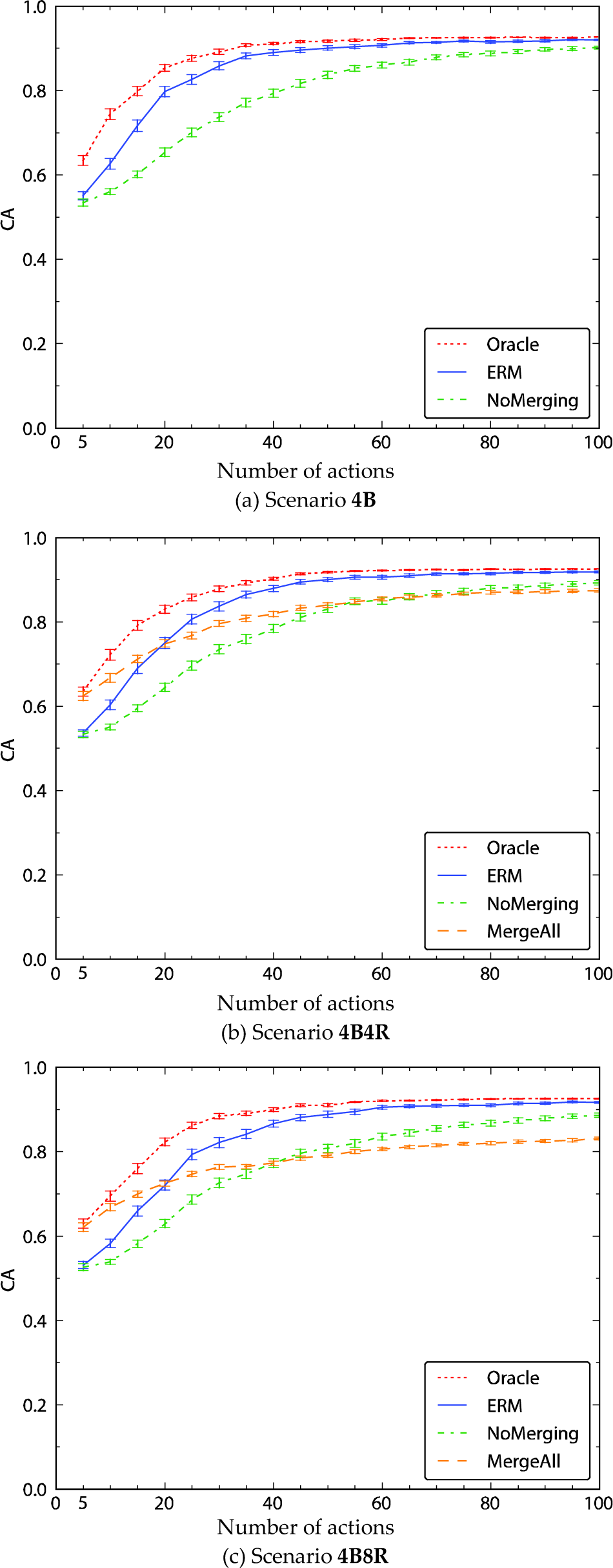
The next question we set ourselves was: “How does the presence of four objects from a different behaviour class affect the speed of learning?” Therefore, we compared the learning curves for scenario with four boxes (4B) with the ones for scenario with four boxes and four other mobile robots (4B4R). The results are shown in Fig. 14(a) and Fig. 14(b), respectively. Our ERM method performs very well in the 4B4R scenario and its performance is nearly as good as in the 4B scenario. Its learning curve is not as steep as before during the first 20 actions, but it still closes the margin to Oracle strategy as quickly as before. This means that our ERM method is successful in recognizing which objects belong to the static behaviour class and merging them to speed up the learning of their models.

Figure 14.

Comparison of the performance of the merging strategies in scenarios with four boxes and an increasing number of other mobile robots (0, 4 and 8). Subfigure (a) is the same as Fig. 13(c) and is repeated here for completeness and easier comparison with the other two subfigures.

It is interesting to observe the learning curve of the MergeAll strategy in Fig. 14(b). Initially, it performed as well as Oracle (which represents the upper bound for the performance) and it stayed significantly better than our ERM strategy until 15 completed actions. From 25 actions on, the ERM surpassed it again and stayed ahead until the end. Compared to the NoMerging strategy, MergeAll performed significantly better for the first 45 actions and it only performed significantly worse from 90 actions on. This result suggests that in cases when the data sets for objects are scarce, it may be beneficial to merge them, regardless of whether or not they actually belong to the same behaviour class.

Even more demanding was the scenario with four boxes and eight other mobile robots (4B8R), for which the results are shown in Fig. 14(c). Again, our ERM method performed very well, achieving significantly better results than the NoMerging strategy. The margin between its learning curve and the upper bound provided by Oracle was only slightly wider than in scenario 4B4R. This demonstrates that our ERM method is able to recognize which objects are boxes (i.e., objects from the static behaviour class), despite doubling the number of other mobile robots (i.e., objects from the moving behaviour class) to eight.

The most notable is the difference in performance of the MergeAll strategy between scenarios 4B4R and 4B8R. It performed significantly worse in the latter. This shows that merging four boxes together with eight other mobile robots significantly deteriorates the learning performance. However, this impact is not the same throughout the learning curve. Interestingly, MergeAll still outperformed both our ERM and NoMerging strategies at the beginning (until 20 actions). This again suggests that in cases when the data sets for objects are scarce, it may be beneficial to merge them, regardless of whether or not they actually belong to the same behaviour class. Furthermore, it hints at a possible new merging algorithm that would initially merge all objects and then gradually eliminate objects that no longer conform to the merged object, as more data for each object becomes available.

6.3. Comparison of distinct base machine learning methods in the 4B8R scenario

The last set of experiments compared how the merging strategies perform with distinct base machine learning methods, namely NBC, C4.5 and SVM. We used our most complex scenario (as defined in section 3.2) with four boxes and eight other mobile robots (4R8B) to analyse their performance. The results are shown in Fig. 15.

Figure 15.

Comparison of the performance of the merging strategies with distinct underlying learning algorithms (NBC, C4.5, SVM) in the 4B8R scenario. Subfigure (a) is the same as Fig. 14(c) and is repeated here for completeness and easier comparison with the other two subfigures.

Generally, the results evidence that our ERM method performs well with all of the base learning methods. With C4.5 it needs more actions to close the gap to the upper bound given by Oracle, meanwhile with SVM it narrows the margin approximately as fast as with NBC.

There is a noticeable fall in the performance of the MergeAll strategy with C4.5, as shown in Fig. 15(b). It only dominates our ERM method for the first five actions and it performs significantly worse from action 15 onward. This may indicate that the C4.5 learning algorithm is more susceptible to the additional conflicting data of objects belonging to the moving behaviour class. However, compared to the NoMerging strategy, the MergeAll performs very similar as with NBC, staying significantly better for the first 30 actions.

Another interesting observation is the very poor performance of the NoMerging strategy with SVM, as shown in Fig. 15(c). In this case, NoMerging strategy performs significantly worse than all other strategies, only catching up with the MergeAll strategy after 90 actions. Furthermore, it does not even come close to both our ERM and the Oracle strategies, the difference in CA measuring more than 0.1 after 100 actions. A plausible explanation for this deviation is the fact that the SVM learning algorithm with our chosen parameters (as described in section 5) needs more examples to train a classifier performing as well as classifiers built by NBC or C4.5. This is further supported by the flatter slopes of learning curves of the other strategies, especially Oracle and ERM, using SVM compared to the ones obtained with NBC or C4.5.

Nonetheless, we have not tried to obtain the optimal learning curves for a particular base machine learning algorithm. Rather, we wanted to observe how the relationships between the merging strategies change when we use a set of distinct base machine learning algorithms. Excluding some minor deviations, the relationships remained the same and thus demonstrate that the merging strategies, in particular our ERM method, are independent of the base machine learning method.

7. Conclusion

In this paper we explored the idea of increasing the learning speed of an autonomous learning agent (e.g., a robot) by learning in a more complex environment. The greater complexity of the environment at any time point offers more observations and the agent can therefore collect more data for learning. This can be beneficial if the domain representing the environment has some structure that allows the merging of data. On the other hand, a more complex domain with more unrelated attributes may just be more confusing for the learner.

We have proposed a new learning method named ERM that automatically discovers similarities in the structure of the domain. It does so by taking the learning sets of objects and training a set of models on selected combinations of these learning sets. By observing the average prediction errors of these models and following a set of criteria for merging, it then merges the objects that are likely to belong to the same behaviour class. For appropriate estimation of prediction errors on different data sets, we introduced a generalized leave-one-out cross-validation method.

Another important feature of the ERM method is that it identifies different types of objects solely from the data measured, when several types of objects are present in a world.

In the experiments with the ERM method in a simple robotic domain we detected the following phenomena:

ERM was capable of discovering structural similarities in the domain, which indeed made the learning faster.

ERM with increased learning times tends to catch up with learning, in which the similarities are already given (i.e., the Oracle merging strategy).

ERM was clearly superior to conventional, unstructured learning (i.e., the NoMerging strategy).

These observed trends occurred with different base machine learning algorithms used inside the ERM method.

One limitation of the presented work is that we have only performed the experiments in one relatively simple domain. We plan to address this in our future work and perform a range of experiments on various different domains and by learning various different relations.

Another limitation of the ERM method is that the agent must know the object–attribute relations (i.e., which measurements belong to which object). By having that information, it can separate one big trace of observations into smaller traces, one for each object it observes. Also, the pair-wise correspondence between attributes of candidate objects for merging must be known.

One interesting observation from our experiments is the surprisingly good performance of the MergeAll strategy at the beginning of the learning process, outperforming our ERM method. This suggests a new learning approach which would initially merge all objects together and then gradually split them apart, as more data for each object becomes available.

In our paper, we chose to minimize the experimentation time (i.e., the number of actions) needed to achieve a certain prediction accuracy. However, depending on the specific robot setting, other criteria may be more appropriate. Different actions by the robot may take different amounts of time, or there may be other kinds of cost associated with each action. In such cases, it would be interesting to try to extend our ERM method to consider more general cost functions. This would also involve the question of optimal choice of actions which is the topic investigated by the areas of active learning and reinforcement learning.

Footnotes

8. Acknowledgements

We would like to thank the Laboratory of Robotics of Faculty of Electrical Engineering at University of Ljubljana for lending us the robots used in .

References

Quinlan

J. R.

, C4.5: Programs for Machine Learning, The Morgan Kaufmann series in machine learning, Morgan Kaufmann, 1993.

Pan

Yang

, A Survey on Transfer Learning, IEEE Transactions on Knowledge and Data Engineering 22 (2010) 1345–1359.

Dai

Yang

Xue

, Boosting for Transfer Learning, in: Proceedings of the twenty-fourth International Conference on Machine learning (ICML), ACM Press, pp. 193–200.

Liao

Xue

Carin

, Logistic Regression with an Auxiliary Data Source, in: Proceedings of the twenty-second International Conference on Machine learning (ICML), ACM Press, pp. 505–512.

Panait

Luke

, Cooperative Multi-Agent Learning: The State of the Art, Autonomous Agents and Multi-Agent Systems 11 (2005) 387–434.

Kelly

Keating

, Faster learning of control parameters through sharing experiences of autonomous mobile robots, International Journal of Systems Science 29 (1998) 783–793.

Buffet

Dutech

Charpillet

, Shaping multi-agent systems with gradient reinforcement learning, Autonomous Agents and Multi-Agent Systems 15 (2007) 197–220.

Sutton

Barto

, Reinforcement learning: an introduction, Adaptive computation and machine learning, MIT Press, 1998.

Dorigo

Colombetti

, Robot Shaping: Developing Autonomous Agents through Learning, Artificial Intelligence 71 (1994) 321–370.

10.

Strehl

Diuk

Littman

, Efficient Structure Learning in Factoredstate MDPs, in: Proceedings of the twenty-second AAAI Conference on Artificial Intelligence, AAAI Press, pp. 645–650.

11.

Diuk

Cohen

Littman

, An Object-Oriented Representation for Efficient Reinforcement Learning, in: Proceedings of the twenty-fifth International Conference on Machine Learning (ICML), ACM Press, pp. 240–247.

12.

Shrager

Langley

, Computational models of scientific discovery and theory formation, The Morgan Kaufmann series in machine learning, Morgan Kaufmann Publishers, 1990.

13.

Langley

, BACON.1: A general discovery system, in: Proceedings of the second National Conference of the Canadian Society for Computational Studies in Intelligence, pp. 173–180.

14.

Langley

, Rediscovering physics with BACON.3, in: Proceedings of the sixth International Joint Conference on Artificial Intelligence (IJCAI), pp. 505–507.

15.

Langley

Bradshaw

Simon

, BACON.5: The discovery of conservation laws, in: Proceedings of the seventh International Joint Conference on Artificial Intelligence (IJCAI), pp. 121–126.

16.

Darden

, Recent Work in Computational Scientific Discovery, in: Proceedings of the nineteenth annual conference of the Cognitive Science Society (CSS), pp. 161–166.

17.

Langley

, The computational support of scientific discovery, International Journal of Human-Computer Studies 53 (2000) 393–410.

18.

Žabkar

Bratko

Mohan

A. C.

, Learning Qualitative Models by an Autonomous Robot, in: Proceedings of the twenty-second International Workshop on Qualitative Reasoning (QR), pp. 150–155.

19.

Hastie

Tibshirani

Friedman

J. H.

, The Elements of Statistical Learning: Data Mining, Inference, and Prediction, Springer series in statistics, Springer, 2009.

20.

Michel

, Webots: Professional Mobile Robot Simulation, Journal of Advanced Robotics Systems 1 (2004) 39–42.

21.

Cortes

Vapnik

, Support-Vector Networks, Machine Learning 20 (1995) 273–297.

22.

Demšar

Zupan

Leban

Curk

, Orange: From Experimental Machine Learning to Interactive Data Mining, in: Boulicaut

J.-F.

Esposito

Giannotti

Pedreschi

(Eds.), Knowledge Discovery in Databases: PKDD 2004, volume 3202 of Lecture Notes in Computer Science, Springer Berlin / Heidelberg, 2004, pp. 537–539.

23.

Cleveland

W. S.

Devlin

, Locally Weighted Regression: An Approach to Regression Analysis by Local Fitting, Journal of the American Statistical Association 83 (1988) 596–610.

Learning Faster by Discovering and Exploiting Object Similarities

Abstract

Keywords

1. Introduction

2. Related work

2.1. Transfer learning

2.2. Cooperative multi-agent learning

2.3. Speeding up reinforcement learning

2.4. Learning by experimentation

3. Experimental domain

3.1. Learning the change in object distance

3.2. Scenarios with worlds of increasing cardinal and behavioural complexity

4. Error reduction merging (ERM)

4.1. Merging objects' data

4.2. Estimating the average prediction errors and significances using a generalized leave-one-out method

4.3. Merging objects using the ERM method

4.4. Learning algorithm running on the robot

5. Experimental setup

6. Experimental results

6.1. Scenarios with an increasing number of boxes

6.2. Scenarios with four boxes and an increasing number of other mobile robots

6.3. Comparison of distinct base machine learning methods in the 4B8R scenario

7. Conclusion

Footnotes

8. Acknowledgements

References