Sage Journals: Discover world-class research

Abstract

Due to event-triggered sampling in a system, or maybe with the aim of reducing data storage, tracking many applications will encounter irregular sampling time. By calculating the matrix exponential using an inverse Laplace transform, this paper transforms the irregular sampling tracking problem to the problem of tracking with time-varying parameters of a system. Using the common Kalman filter, the developed method is used to track a target for the simulated trajectory and video tracking. The results of simulation experiments have shown that it can obtain good estimation performance even at a very high irregular rate of measurement sampling time.

Keywords

Target Tracking Irregular Sampling Time Kalman Filter Irregular Rate State Estimation

1. Introduction

Tracking a variable number of interest targets has been applied many fields, such as self-navigating robots, video surveillance applications, etc. Classical tracking methods using a single sensor involve a dynamics model of manoeuvring the target and state estimation based on measurements obtained system's sensor. In general, the Kalman filter [1 –4] and particle filter [5, 6] are the most commonly used estimation methods. It is well-known that the discrete Kalman filter has the advantages of simple and recursive calculation. Though the Kalman filter cannot obtain good performance while the system noises are not Gaussian white noise, it is the most widely used method in target tracking. The discrete Kalman filter and its improved form based on different applications, such as the system with nonlinear measurement (named the extended Kalman filter or unscented Kalman filter) is a classic problem with a long and continuing history of research.

We know the movement of a target is based on the continuous relation of location, velocity and acceleration. But the system can only obtain discrete sampling measurements, so in general the continuous dynamic model is discretized based on assumptions using same sampling time interval and the Kalman filter recursively estimates the state of the system based on sampling measurements from K to K +1. But if the output measurements are sampled on a set of non-periodic and irregular sampling times, or the sampled values are lost when they are transmitted, the traditional recursive estimation from K to K +1 may fail in general, even if the system has a full-rank measurement matrix.

While synchronized periodic sampling has been studied, non-uniform sampling has emerged from many applications. Most event-triggered sampling systems can generate irregular sampling time sequences. For example, in the supply chain system [7], radio frequency identification (RFID) technologies can automatically record the location of specific items at the time when these are within a reader's range. So if we want to estimate the item's target by the record measurements, we must deal with the estimation problem based on irregular sampling.

The main challenges in target tracking under irregular sampling include: 1) when will the sampled system be observable under irregular sampling sequences? 2) How to estimate the target trajectory on the basis of irregular sampling points. 3) What convergence properties can be derived for the state estimates? This paper focuses on these problems and is organized as follows. Section II discusses some research results about estimation with irregular sampling measurements. Section III formulates the target tracking problems pursued in this paper. Section IV focuses on the observability of systems under arbitrary sampling times. Section V gives the dynamic model under the irregular sampling time and the estimation method based on the Kalman filter. A simulation example is provided in Section VI. Finally, some concluding remarks are given in Section VII.

2. Related Works

As a state estimation problem for continuous processes with discrete measurements, there are three approaches as follows[8]:

Approach 1)

For the discrete measurement and its sampling time, the continuous process model is discretized. After that, one of the known state estimators for discrete systems is applied to obtain state estimates of a continuous process at discrete moments.

Approach 2)

The second alternative is to lift the discrete measurements into the space of continuous functions (e.g., by using a polynomial fit of several discrete measurements in a sliding window) and then apply one of the known state estimators for continuous systems, such as the Kalman-Bucy filter.

Approach 3)

The final option is to directly consider the state estimation problem with a continuous model and an arbitrary combination of discrete and continuous measurements. This approach is more difficult theoretically because it leads to a continuous filter with discontinuous inputs.

The application of the discrete Kalman filter (or extended Kalman filter or unscented Kalman filter) to estimate states of continuous stochastic systems is common. [9, 10] deal with state estimation in the presence of delayed and infrequent measurements under a common unified extended Kalman filter framework. [10, 11] discuss some related issues of non-uniformly sampled systems, including model derivation, controllability and observability, computation of single-rate models with different sampling periods, reconstruction of continuous-time systems, and parameter identification of non-uniformly sampled discrete-time systems. [12] introduces a method of designing observers for linear time invariant systems with irregular sampling time sequences, which can be generated either passively in event-triggered sampling or by actively controlling the system input or sensor threshold when the sensor is binary-valued. Studies on Approach 2) remain an active area of research, see [13 –16] and the references therein for some recent work in this area. [8] follows Approach 3) and develops the optimal state estimation for continuous and sampled measurements using the theory of vibrosolutions.

In this paper, we follow Approach 1). We note that the results about estimation methods of the discrete Kalman filter for irregular sampling[12] cannot be used for the target tracking problem directly. For example, the matrix exponential of A, i.e., e^A is obtained by a polynomial function of A based on the Cayley-Hamilton theorem in [12], which requires A to be a full-rank matrix. But we know this condition does not hold for a target tracking system. Another new problem we must face is there is not input signal, and here we must deal with the system noise, including processing noise and measurement noise, which is not very common in the estimation problem of a control system. Therefore, for the target tracking problem, we must calculate e^A for a not-full-rank matrix and discretize system noise under irregular sampling. These problems will be solved in this paper.

3. System model and problem formulation

It is known that the target problem involves the dynamics model, so here we begin with several models of target manoeuvring. The first common model is the Singer model[17 –19], in which models target acceleration as a first-order semi-Markov process with zero mean. It is in essence an a priori model since it does not use online information about the target manoeuvre, although it can be made adaptive through an adaptation of some parameters. Due to the complexity of the actual target, no a priori model can be remarkably effective in the diverse acceleration situations of actual target manoeuvres. One of the main shortcomings of the Singer model is that the target acceleration has zero mean at any moment. Another shortcoming is that the Singer model cannot use online information.

An acceleration model, called the “current model”[20] is in essence a Singer model with an adaptive mean; that is, a Singer model modified to have a non-zero mean of the acceleration. In the “current model”, the model can use online information of tracking, and a priori (unconditional) probability density of the acceleration in the Singer model is replaced by a conditional density, i.e., Rayleigh density. Clearly, this conditional density carries more accurate information and is better to use than a priori density. We note that this conditional Rayleigh assumption was made for the sole purpose of obtaining the variance of the acceleration prediction.

Let x, ẋ and ẍ be the target position, velocity and acceleration along a generic direction, respectively – specifically, ẍ(t) = a(t). In this section, the state vector is always taken to be x = [x,ẋ,ẍ]', unless explicitly stated otherwise. We use a non-zero-mean acceleration the same as the “current model”[20], which satisfies ẍ(t) = ā + a(t), where

\dot{a} (t) = - α a (t) + w (t)

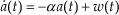
where a(t) is zero-mean first-order stationary Markov process, i.e., the acceleration of the target with variance δ²_a, ā; is the mean of acceleration a(t) and w(t) is zero-mean white noise with variance δ²_w = 2αδ²_a. Let a₁(t) = ā + a(t), we have

\begin{array}{l} \ddot{x} (t) = a_{1} (t) \\ {\dot{a}}_{1} (t) = - α a_{1} (t) + α \bar{a} + w (t) \end{array}

The state-space representation of the continuous-time adaptive model is

\dot{x} (t) = [\begin{matrix} 0 & 1 & 0 \\ 0 & 0 & 1 \\ 0 & 0 & - α \end{matrix}] x (t) + [\begin{matrix} 0 \\ 0 \\ α \end{matrix}] \bar{a} (t) + [\begin{matrix} 0 \\ 0 \\ 1 \end{matrix}] w (t)

(1)

Note that in the “current model”, this conditional Rayleigh assumption was made for the sole purpose of obtaining the variance of the acceleration prediction, which turns out to be

δ_{a}^{2} = {\begin{matrix} \frac{4 - π}{π} {(α_{\max} - {\hat{a}}_{k})}^{2} {\hat{α}}_{k} > 0 \\ \frac{4 - π}{π} {(α_{- \max} + {\hat{a}}_{k})}^{2} {\hat{α}}_{k} < 0 \end{matrix}

Parameter α is called the “manoeuvring frequency”, which can be obtained by estimating online or by assuming that the appropriate value based on experience. Studies on the value of α remain active areas of research, see and the references [21 –23]therein for some recent work in this area.

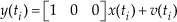
The continuous measurement model is as follows:

y (t) = [\begin{matrix} 1 & 0 & 0 \end{matrix}] x (t) + v (t)

But we can only obtain the discrete measurement values at the sampling time t_i and at the sampling time we have the discrete measurement model as:

y (t_{i}) = [\begin{matrix} 1 & 0 & 0 \end{matrix}] x (t_{i}) + v (t_{i})

(2)

Now considering (1) and (2), we have the following hybrid system dynamics equation as follows:

\dot{x} (t) = A x (t) + U \bar{a} (t) + B w (t)

(3)

y (t_{i}) = C x (t_{i}) + v (t_{i}), i = \begin{matrix} 1, & 2, & \dots & N \end{matrix}

(4)

where

A = [\begin{matrix} 0 & 1 & 0 \\ 0 & 0 & 1 \\ 0 & 0 & - α \end{matrix}], U = [\begin{matrix} 0 \\ 0 \\ α \end{matrix}], B = [\begin{matrix} 0 \\ 0 \\ 1 \end{matrix}], C = [\begin{matrix} 1 & 0 & 0 \end{matrix}]

(5)

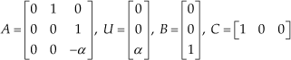
and w(t)and v(t_i) are process and measurement noise, respectively. They are uncorrelated at each sampling time, with the covariance matrix given by w(t) ∼ N(0,2αδ_a²) and E{v(t_k)v^T(t_j)} = R(t_k)δ_kj, where E denotes expectation, δ_kj is the Kronecher delta, R(t_k) is positive definite.

The target tracking problem is described as follows: given the system model of manoeuvring target as (3), we would like to estimate the state x(t_i) from the information based on y(t_i)and v(t_i) at irregular sampling time t_i with the measurement model (4).

4. Observability of the target system under irregular sampling

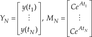
We start with the system in (3) and (4) with noise-free measurement, i.e., w(t) = 0 and v(t_i) = 0. Suppose that the output of the system is sampled at a set of N time instances T_N={t_i ≥ 0, i = 1, …, N}. Observability of the sampled system deals with reconstruction of the state x(t) from output measurements ϒ _N = {y(t_i), i = 1,…N}. Since the system contains no uncertainty, this is equivalent to reconstruction of the initial state x(t) from ϒY _N .

The solution of differential equations (3) is

x (t) = e^{_{^{A t}}} x (0) + \int_{0}^{t} e^{A t} U \bar{a} (λ) d λ + \int_{0}^{t} e^{A t} B w (λ) d λ, t \geq 0

Without loss of generality, we may focus only on the zero-input relationship y(t) = Ce^Atx(0). Under N sampling times T _N = {t_i ≥ 0, i = 1, …, N}, we have ϒ _N = {y(t_i), i = 1,…N} with y(t_i) = Ce^Atix(0), i = 1,…N, which can be written as Y_N = M_Nx(0), where

Y_{N} = [\begin{matrix} y (t_{1}) \\ ⋮ \\ y (t_{N}) \end{matrix}], M_{N} = [\begin{matrix} C e^{A t_{1}} \\ ⋮ \\ C e^{A t_{N}} \end{matrix}]

Because the process matrix of system A in (5) is not a full-rank matrix, we cannot calculate the matrix exponential e^Ati using the Lagrange-Hermite interpolation[12], therefore we use the Laplace transform giving

{(s I - A)}^{- 1} = {[\begin{matrix} s & - 1 & 0 \\ 0 & s & - 1 \\ 0 & 0 & s + α \end{matrix}]}^{- 1} = [\begin{matrix} \frac{1}{s} & \frac{1}{s^{2}} & \frac{1}{s^{2} (s + α)} \\ 0 & \frac{1}{s} & \frac{1}{s (s + α)} \\ 0 & 0 & \frac{1}{s + α} \end{matrix}]

The matrix exponential e^Ati is obtained by using the inverse Laplace transform as follows:

e^{A t_{i}} = [\begin{matrix} 1 & t_{i} & \frac{α t_{i} - 1 + e^{- α t_{i}}}{α^{2}} \\ 0 & 1 & \frac{1 - e^{- α t_{i}}}{α} \\ 0 & 0 & e^{- α t_{i}} \end{matrix}]

(6)

Then we have

M_{N} = [\begin{matrix} 1 & t_{1} & \frac{α t_{1} - 1 + e^{- α t_{_{2}}}}{α^{2}} \\ ⋮ & ⋮ & ⋮ \\ 1 & t_{N} & \frac{α t_{N} - 1 + e^{- α t_{_{N}}}}{α^{2}} \end{matrix}]

We know for any t_i, i ≥ 1, M_N must be a full-rank matrix. That means the system is observable when there are i sampling measurements (i ≥ 1). But we know there are noises in the process and measurement system, so the effective estimation method needs to overcome the influence of noise to obtain the exact estimation of the real state.

5. Estimation method under irregular sampling

Now we consider the time interval from t_i-1 to t_i and we have the state variation from t_i-1 to t_i as

x (t_{i}) = e^{^{A (t_{i} - t_{i - 1})}} x (t_{i - 1}) + \int_{t_{i - 1}}^{t_{i}} e^{A (t_{i} - t_{i - 1})} U \bar{a} (λ) d λ + \int_{t_{i - 1}}^{t_{i}} e^{A (t_{i} - t_{i - 1})} B w (λ) d λ .

Denote t_hi = t_i – t_i-1 and we have

x (t_{i}) = e^{^{A t_{h i}}} x (t_{i - 1}) + \int_{t_{i - 1}}^{t_{i}} e^{A t_{h i}} U \bar{a} (λ) d λ + \int_{t_{i - 1}}^{t_{i}} e^{A t_{h i}} B w (λ) d λ

(7)

For the right part of (7), we assume ā(λ) = ā(t_i-1), w(λ) = w(t_i–1), λ ∈[t_-1 t_i], then we have

\int_{t_{i - 1}}^{t_{i}} e^{A t_{h i}} U \bar{a} (λ) d λ = \int_{t_{i - 1}}^{t_{i}} e^{A t_{h i}} U d λ \bar{a} (t_{i - 1})

and

\int_{t_{i - 1}}^{t_{i}} e^{A t_{h i}} B w (λ) d λ = \int_{t_{i - 1}}^{t_{i}} e^{A t_{h i}} B d λ w (t_{i - 1}) .

So using a similar approach and by using the inverse Laplace transform we get (6), and we can now obtain the discrete process model at the sampling time as follows:

x (t_{i}) = A_{d} (t_{i - 1}) x (t_{i - 1}) + U_{d} (t_{i - 1}) \bar{a} (t_{i - 1}) + w_{d} (t_{i - 1})

(8)

where

\begin{matrix} A_{d} (t_{i - 1}) = [\begin{matrix} 1 & t h_{i} & \frac{α t h_{i} - 1 + e^{- α t h_{i}}}{α^{2}} \\ 0 & 1 & \frac{1 - e^{- α t h_{i}}}{α} \\ 0 & 0 & e^{- α t h_{i}} \end{matrix}] \\ U_{d} (t_{i - 1}) = [\begin{matrix} \frac{1}{α} (- t h_{i} + \frac{α \cdot t h_{i}^{2}}{2} + \frac{1 - e^{- α \cdot t h_{i}}}{α}) \\ t h_{i} - \frac{1 - e^{- α \cdot t h_{i}}}{α} \\ 1 - e^{- α \cdot t h_{i}} \end{matrix}] \end{matrix}

Q_{d} (t_{i - 1}) = E [w_{d} (t_{i - 1}) w_{d}^{T} (t_{i - 1})] = 2 α δ_{α}^{2} [\begin{matrix} q_{11} & q_{12} & q_{13} \\ q_{12} & q_{22} & q_{23} \\ q_{13} & q_{23} & q_{33} \end{matrix}]

(9)

\begin{array}{l} q_{11} = \frac{1}{2 α^{5}} [1 - e^{- 2 α \cdot t h_{i}} + 2 α \cdot t h_{i} + \frac{2 α^{3} t h_{i}^{3}}{3} - 2 α^{2} t h_{i}^{2} - 4 α \cdot t h_{i} e^{- α \cdot t h_{i}}] \\ q_{12} = \frac{1}{2 α^{4}} [e^{- 2 α \cdot t h_{i}} + 1 - 2 e^{- α \cdot t h_{i}} + 2 α \cdot t h_{i} e^{- α \cdot t h_{i}} - 2 α \cdot t h_{i} + α^{2} t h_{i}^{2}] \\ q_{13} = \frac{1}{2 α^{3}} [1 - e^{- 2 α \cdot t h_{i}} - 2 α \cdot t h_{i} e^{- α \cdot t h_{i}}] \\ q_{22} = \frac{1}{2 α^{3}} [4 e^{- α \cdot t h_{i}} - 3 - e^{- 2 α \cdot t h_{i}} + 2 α \cdot t h_{i}] \\ q_{23} = \frac{1}{2 α^{2}} [e^{- 2 α \cdot t h_{i}} + 1 - 2 α \cdot t h_{i}] \\ q_{33} = \frac{1}{2 α} [1 - e^{- 2 α \cdot t h_{i}}] \end{array}

Until now, the irregular sampling has been turned to the varying system parameter shown in (9). From (8) and (9), we can see that the irregular sampling time t_i, t_i-1 and irregular sampling interval t_hi are the main part of the system parameters A_d, U_d and Q_d. The parameters t_i, t_i-1 and t_hi describe how sparse and irregular data could be in the irregular system. To illustrate the influence of the sampling irregularities on the system performance, we arrive at the following lemma.

Lemma 1: Given the continuous system dynamics (3), we can have the discrete system Equation (8) with parameters described as (9) for any known sampling time t_i-1 and t_i.

Proof: We begin with solving the state x(t) of the differential (3).

For the exponential function e^At, we have

e^{A t} = I + A t + \frac{A^{2} t^{2}}{2!} + \frac{A^{3} t^{3}}{3!} + \frac{A^{4} t^{4}}{4!} + \dots \dots .

and

\frac{d}{d t} e^{A t} = A + A^{2} t + \frac{A^{3} t^{2}}{2!} + \frac{A^{4} t^{3}}{3!} + \frac{A^{5} t^{4}}{4!} + \dots \dots = A \cdot e^{A t}

(10)

\frac{d}{d t} [e^{- A t} x (t)] = e^{- A t} [\dot{x} (t) - A \cdot x (t)]

(11)

By left multiplying e^−At on both sides of (3), we can get

e^{- A t} [\dot{x} (t) - A \cdot x (t)] = e^{- A t} U \bar{a} (t) + e^{- A t} B w (t)

(12)

By using (11), we can know the left of (12) is $\frac{d}{d t} [e^{- A t} x (t)]$ , then we have the following:

\frac{d}{d t} [e^{- A t} x (t)] = e^{- A t} U \bar{a} (t) + e^{- A t} B w (t)

(13)

For solving integrating both sides of (13) and setting integration interval as [t₀, t], we can obtain

e^{- A t} x (t) = e^{- A t_{0}} x (t_{0}) + \int_{t_{0}}^{t} e^{- A λ} U \bar{a} (λ) d λ + \int_{t_{0}}^{t} e^{- A λ} B w (λ) d λ

(14)

Left multiply e^−At on both sides of (14), we have

x (t) = e^{A (t}^{- t_{0})} x (t_{0}) + \int_{t_{0}}^{t} e^{A (t - λ)} U \bar{a} (λ) d λ + \int_{t_{0}}^{t} e^{A (t - λ)} B w (λ) d λ

(15)

Then we can conclude that for any known integration interval as [t₀, t], if we only know the initial state x(t₀) and the parameter A, U, B and ā(t), and w(t) in [t₀, t], we can use (15) to get x(t) at time t.

Now we set the sampling time as t_i = t and t_i-1 = t₀. We know if the state x(t₁) and the parameter A, U, B and ā(t), and w(t)in [t_i-1, t_i], are known, then the state x(t_i) can be obtained only if under the condition that the sampling time t_i-1 and t_i are known.

For the process model (8) and measurement model (4) with the system parameter (9), we use the Kalman filter to get the estimate of system state at every sampling time as follows:

Initialization: i = 0

\hat{x} (t_{0} | t_{0}) = x_{0} P (t_{0} | t_{0}) = P_{0} δ_{w}^{2} (t_{0}) = δ_{w 0}^{2}

(16)

Recursion: i:=i+1

Prediction:

\hat{x} (t_{i} | t_{i - 1}) = A_{d} (t_{i - 1}) \hat{x} (t_{i - 1} | t_{i - 1}) + U_{d} (t_{i - 1}) \bar{a}

(17)

P (t_{i} | t_{i - 1}) = A_{d} (t_{i - 1}) P (t_{i - 1} | t_{i - 1}) A_{d}^{T} (t_{i - 1}) + Q_{d} (t_{i - 1})

(18)

State update:

\hat{x} (t_{i} | t_{i}) = \hat{x} (t_{i} | t_{i - 1}) + K (t_{i}) [y (t_{i}) - C (t_{i}) \hat{x} (t_{i} | t_{i - 1})]

(19)

K (t_{i}) = P (t_{i} | t_{i - 1}) H^{T} (t_{i}) {[H (t_{i}) P (t_{i} | t_{i - 1}) H^{T} (t_{i}) + R (t_{i})]}^{T}

(20)

P (t_{i} | t_{i}) = [I - K (t_{i}) H (t_{i})] P (t_{i} | t_{i - 1})

(21)

The filter can get the estimation of state update at t_i by (16) to (21). We know the estimation performance obtained by the Kalman filter is based on whether the model is in accordance with the real moving target characteristics. For the estimation problem with the regular sampling time, if the system parameters A_d, U_d, Q_d, C and R are consistent with the actual status of the system, the Kalman filter can obtain the optimal estimation performance. But for the real tracking problem, the covariance of process noise w(t) is very difficult to model. This paper uses the “current model” with w(t) ∼ N(0,2αδ²) discussed in Section III and the value of parameter α and δ² _a can affect the estimation performance. The more accurate the parameters used, the better the performance. As for the effect of irregular sampling on the estimated performance, we have the following theorem:

Theorem 1: The Kalman filter shown in (16)-(21) based on the system (3) and (4) under the irregular sampling time with time-varying system parameters (9) can obtain the same estimation performance as regular sampling time.

Proof: Because the irregular sampling is turned to the varying system parameter and the Kalman filter is just based on the variable parameter of the system, we can abbreviate t_i to i and t_i-1 to i-1. The Kalman filter (16)-(21) is just like the common Kalman filter, so the details of the proof process are omitted here.

6. Simulation results

Define 1. The irregular rate is to measure the sampling time as follows:

I R r a t e = \frac{\sum_{i = 1}^{N} | t h_{i} - \sum_{i = 1}^{N} t h_{i} |}{N}

The following simulations are to show the relation of the irregular rate and estimation performance. Firstly, the target moves along the attenuation of the sinusoidal movement (Scenario I), and the measurement noises are generated as white Gaussian random numbers with variance R. We assume R is a given parameter, which can be obtained in most tracking systems, R = 2 and the manoeuvring frequency α and α_max of the “current model” is set to be $\frac{1}{10}$ and 30. The estimation results and errors are shown in Figure 1(a) and (b). We note that the sampling time intervals are different to those shown in Figure 1(c) and the biggest sampling interval and the irregular rate of the measurement sampling time is 0.6766 and 0.0418. We can also obtain the estimation covariance as 2.1181 for the location estimation and the covariance matrix obtained by the Kalman filter is

Figure 1.

The estimate results with measurements of sinusoidal movement (a) the real state and estimate; (b) the estimate error; (c) the interval between the current and previous sampling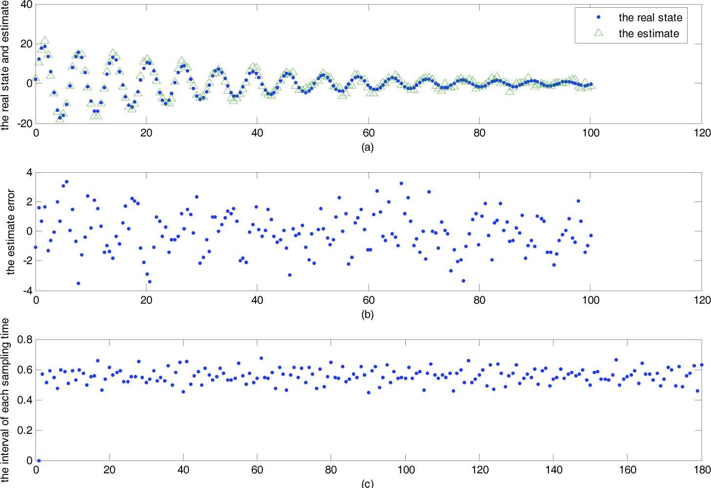

[\begin{matrix} 1.7757 & 2.8245 & 2.1640 \\ 2.8245 & 10.9597 & 15.3735 \\ 2.1640 & 15.3735 & 36.8871 \end{matrix}]

To further illustrate how the irregular rate affects estimation performance, the algorithm is used to estimate the target trajectory under different irregular rates. After 100 Monte Carlo simulation runs, the root-mean square errors (RMSE) of position are calculated with the irregular rate, which is shown in Table 1.

Table 1.

Comparison of the Estimation Results

	Case 1	Case 2	Case 3	Case 4	Case 5	Case 6	Case 7	Case 8
the root-mean square errors (RMSE) of position	2.0308	2.0487	2.0453	2.0429	2.0385	2.0407	2.0738	2.0556
the irregular rate	0	0.0085	0.0176	0.0304	0.0456	0.0543	0.0661	0.0890

From the table, we can see that the irregular rate affects the estimation performance very little. The irregular rate changes ten times from 0.0085 in Case 2 to 0.0890 in Case 8, but the estimation performance has almost no change (root-mean square errors (RMSE) of position is almost always 2.04), just like a system with regular sampling time (in Case 1).

To further study the effect of irregular sampling on the estimation performance, we use the square wave as the trajectory of the moving target and we note this case as Scenario II. Firstly the regular sampling measurement is tracked (shown in Figure 2(a) by the “circle”) and the sampling time is 0.625s. The estimation results get are shown in Figure 2(a) with the “star”, and the estimation error obtained is shown as in Figure 2(b). The covariance of estimation is 30.7838 for the location estimation. From Figure 2, we can see the estimation error becomes large when the trajectory makes dramatic changes, for example, at 9 and 17 sampling points (the sampling times are 5.625s and 10.625s, respectively), and the estimation errors are −11.3116 and 9.5931, respectively. The reason for this is because the acceleration components in square wave undergo dramatic changes, exceeding the model noise modelling capabilities of the “current model”, i.e., Rayleigh distribution in the “current model” discussed in Section III cannot accurately describe the acceleration distribution of square wave trajectory.

Figure 2.

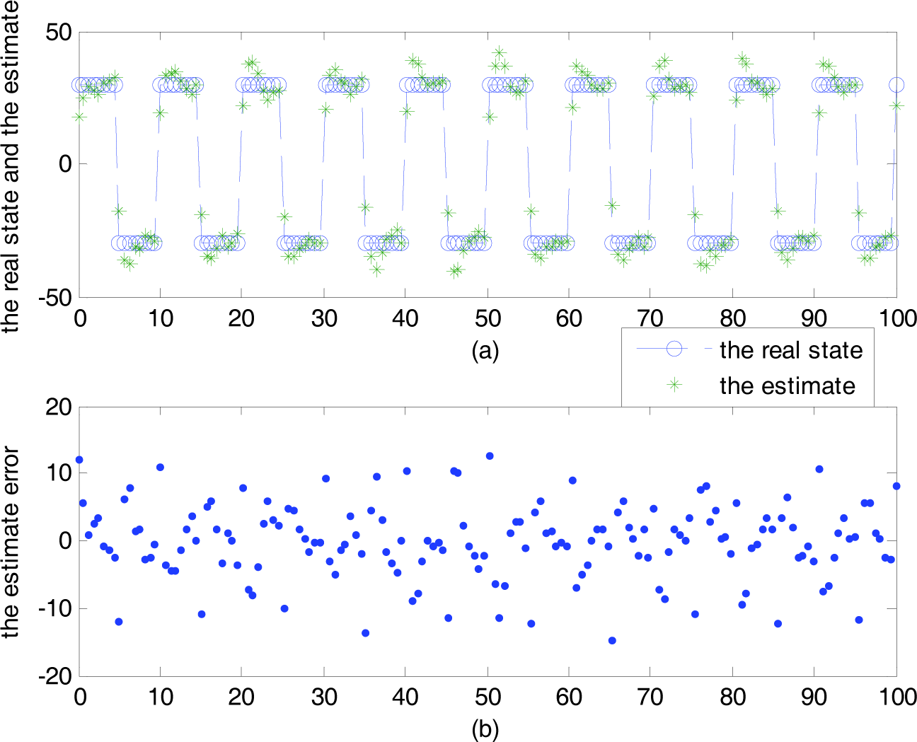
The estimate results with regular sampling for square wave movement (a) the real state and estimate; (b) the estimate error

Then we use the same number of sampling points (160 sampling points in 100s), but irregular sampling time for the square trajectory with the irregular rate 0.5119. The square wave trajectory and the estimate, the estimation error and the sampling time intervals at every sampling are shown in Figure 3(a), (b) and (c). The estimation covariance is 24.0456 with 100 Monte Carlo simulations.

Figure 3.

The estimate results with irregular sampling for square wave movement (a) the real state and estimate; (b) the estimate error; (c) the interval of each sampling time

We note that the irregular sampling time in Figure 3 obtained the smaller estimation covariance compared to the regular sampling time in Figure 2. We analyse the reasons as follows:

We know for the regular sampling time tracking problems, the estimation performance is decided by the accuracy of the model and the robustness of the estimation method for the model. From Figure 2 we can see the error occurs mainly in the dramatic changes of the trajectory. As to the irregular sampling case in Figure 3, we notice that the number of dramatic changes is reduced, as indicated by 1, which is no longer vertical (for example, indicated by 2), but has a certain slope. Therefore the error in the point indicated by 1 is smaller.

On the other hand, the estimation error does not increase due to the variation of the sampling interval. As proven in Lemma 1, the irregular sampling cannot decrease the estimation performance. Therefore the estimation performance is better in Figure 3 and simulation results are consistent with the theory proved in Theorem 1.

For a more practical view, the method here is applied to a two dimensional planar video tracking (Scenario III). Here, as a tracking problem, we just use the simple background and one target. The video obtained by the Image Capture Test Bed is shown in Figure 4. Extracting the target from a complex background in a video image, tracking multiple targets or tracking by multi-sensor will not be discussed here.

Figure 4.

The video with simple background and one target

We control the car manoeuvring on the test bed and catch the images of the movement of the target by using a stationary camera. For every image of the video, the target is extracted based on the colour, then we get the trajectory data of the manoeuvring target on the Image Capture Test Bed as in Figure 5.

Figure 5.

The trajectory of the manoeuvring target obtained from the video

We know the camera captures the image under the same interval, and that will produce large amounts of image data. So if we can use the part of the images in the video for the tracking of the target with the good performance, the image storage and computation cost will be greatly reduced. But “using the part of images” means that the system no longer has the same sampling interval. Here we randomly extract part of the video images and define the extraction rate as

E x r a t e = \frac{extracted images from the video}{total images in the video} \times 100 %

to descript the image compression rate.

The extraction images have irregular sampling time and the target is tracked to illustrate the effectiveness of the method developed here. The initial condition for the target with state

x (k) = [\begin{matrix} x (k) & \dot{x} (k) & \ddot{x} (k) & y (k) & \dot{y} (k) & \ddot{y} (k) \end{matrix}] .

The initial state estimate x₀ and covariance P₀ are assumed to be x₀ = [0 0 0 0 0 0]' and P₀=diag(10,10,10,10,10,10).

We extract 59 images from a video with 111 images and get the estimation of trajectory with estimation covariance 4.1078 (the horizontal axis) and 5.2511 (the vertical axis), and the irregular rate 0.0927, as shown in Figure 6. The estimation errors are shown in Figure 7. Some other estimation results are shown in Figure 8, and the data on estimation covariance and irregular rate, etc., are in Table 2.

Table 2.

The estimation covariance and irregular rate in the Figure 8

Video in Figure 6	total images in the video	extracted images from the video	extraction rate	estimation covariance (horizontal axis)	estimation covariance (vertical axis)	irregular rate
(a)	191	99	51.83%	1.1256	1.6197	0.1056
(b)	131	62	47.69%	1.0873	3.5923	0.0962
(c)	201	73	36.32%	1.2575	1.4357	0.1535
(d)	271	69	25.46%	1.4422	1.3584	0.2332
(e)	281	33	11.73%	1.5683	1.6710	0.5609
(f)	281	20	7.11%	1.6282	1.7607	1.2554

Figure 6.

The estimation of trajectory

Figure 7.

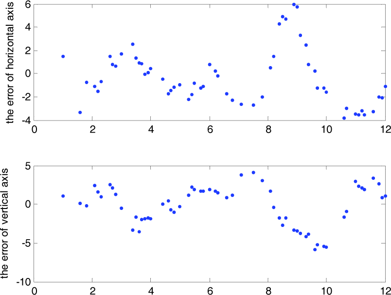
The estimation error in the horizontal axis and vertical axis

Figure 8.

The estimation results for videos

From Figure 8 and the estimation covariance in Table 2, we can see for almost any extraction rate, the estimation performance almost always remained at good levels, even when the extraction rate is 7.11% and the irregular rate is 1.2554 (in Figure 8 (f)). We note that in Figure 8(f), the estimated images are so small that is no longer satisfy the sampling theorem, so from the estimate of state point at sampling time we cannot describe the whole trajectory (we have to show it as a dashed line). But we can still get good estimation performance with 1.6282 and 1.7607 (see Table 2). We can conclude that only if the exacted data contain the recoverability information of the original trajectory, can the method developed here deal with the irregular sampling problem perfectly and the system obtain good estimation performance.

7. Conclusions

Tracking trajectory under irregular sampling time is a common situation, sometimes due to event-triggered sampling in the system, or maybe with the aim of reducing the data storage and computation cost. This paper offers a method to calculate the discrete system model at each sampling time. The matrix factorization method is not used, which is used generally to calculate the matrix exponential, while this paper obtains the process model and measurement model by using the inverse Laplace transform. The estimate is obtained by using the Kalman filter in this paper, which can also be substituted by other estimation methods, such as particle filter, because the affect of irregular sampling time has been transformed into time-varying parameters of the system and the tracking problem here is also a common one which has been extensively studied.

We also note that the method can obtain good estimation performance at all sampling times. So if we want obtain the real trajectory, the only thing we have to do is obtain the appropriate amount of data to describe it. In the usual sense, enough data should be included to satisfy the Shannon sampling theorem. The recently emerged idea of compressive sensing (CS) theory provides a different perspective in solving large underdetermined problems, exploiting sparsity as a prior value. This powerful and promising tool has proven to be effective for a wide range of problems of this class, including sub-Nyquist sensing of signals and coding, image denoising and de-blurring. So one of our future research subjects is how can we use the method of this paper on CS data and get a more complete description of the trajectory in the sub-continuous space, which means by interpolating the discrete trajectory to obtain the approximate discrete description of the original continuous trajectory.

If we do not need to obtain the whole trajectory of the target, and only need to obtain the location, speed and acceleration at some of the sampling points, the method developed here is a good choice. We can see that the estimation performance is perfect, the same as the common Kalman filter, if we know the sampling time, which case often occurs in the actual tracking system.

It is also noticed that we should choose an adaptive model for the tracking and in this paper the “current model” is used. For the “current model”, we need to assume the manoeuvring frequency α and α_max as a given parameter, and we also note that different value of these two parameters will obtain different estimation covariance. Sometimes one parameter can obtain better performance for estimating one trajectory, while maybe not for another trajectory. One of the reasons for this phenomenon is that the system is open-loop for the model parameters, i.e., the system model cannot adapt the movement characteristics of the manoeuvring target. In our opinion, tracking while identifying may be a good solution. That means the close-loop mechanism for the model parameters should be established, which will be one area of future research.

Footnotes

8. Acknowledgements

This work was supported in part by NSFC under grant no. 61273002 and 60971119.

References

Ahn

H. S.

Kim

Y. S.

, and Chen

(2012) An interval Kalman filtering with minimal conservatism. Applied Mathematics and Computation. 218: 9563–9570.

Desbouvries

Petetin

, and Ait-El-Fquih

(2011) Direct, prediction- and smoothing-based Kalman and particle filter algorithms. Signal Processing, 91: 2064–2077.

Godinez

H. C.

, and Moulton

J. D.

(2012) An efficient matrix-free algorithm for the ensemble Kalman filter. Computational Geosciences. 16: 565–575.

Ran

C. J.

, and Deng

Z. L.

(2012) Self-tuning weighted measurement fusion Kalman filtering algorithm. Computational Statistics & Data Analysis. 56: 2112–2128.

X. L.

Schon

T. B.

, and Ljung

(2011) A General Convergence Result for Particle Filtering. IEEE Transactions on Signal Processing. 59: 3424–3429.

T. C.

Sattar

T. P.

, and Sun

S. D.

(2012) Deterministic resampling: Unbiased sampling to avoid sample impoverishment in particle filters. Signal Processing. 92: 1637–1645.

Kelepouris

Harrison

, and McFarlane

(2011) Bayesian Supply Chain Tracking Using Serial-Level Information. IEEE Transactions on Systems Man and Cybernetics Part C-Applications and Reviews. 41: 733–742.

Zhang

H. H.

Basin

M. V.

, and Skliar

(2007) Ito-Volterra optimal state estimation with continuous, multirate, randomly sampled, and delayed measurements. IEEE Transactions on Automatic Control. 52: 401–416

Gopalakrishnan

Kaisare

N. S.

, and Narasimhan

(2011) Incorporating delayed and infrequent measurements in Extended Kalman Filter based nonlinear state estimation. Journal of Process Control. 21: 119–129.

10.

Shah

S. L.

, and Xiao

(2008) Kalman filters in non-uniformly sampled multirate systems: For FDI and beyond. Automatica. 44: 199–208.

11.

Ding

Qiu

, and Chen

T. W.

(2009) Reconstruction of continuous-time systems from their non-uniformly sampled discrete-time systems. Automatica. 45: 324–332.

12.

Wang

L. Y.

C. Y.

Yin

G. G.

(2011) State Observability and Observers of Linear-Time-Invariant Systems Under Irregular Sampling and Sensor Limitations. IEEE Transactions on Automatic Control. 56: 2639–2654.

13.

Bell

B. M.

Burke

J. V.

, and Pillonetto

(2009) An inequality constrained nonlinear Kalman-Bucy smoother by interior point likelihood maximization. Automatica. 45: 25–33

14.

Heydari

Salarieh

, and Behzad

(2011) Stochastic chaos synchronization using Unscented Kalman-Bucy Filter and sliding mode control. Mathematics and Computers in Simulation. 81: 1770–1784.

15.

G. D.

(2008) Symplectic Runge-Kutta methods for the Kalman-Bucy filter. IMA Journal of Mathematical Control and Information. 25: 173–183.

16.

Wang

G. C.

, and Wu

(2008) Kalman-Bucy filtering equations of forward and backward stochastic systems and applications to recursive optimal control problems. Journal of Mathematical Analysis and Applications. 342: 1280–1296.

17.

Chen

Pang

(2010) AUV sensor fault diagnosis based on STF-Singer model. Chinese Journal of Scientific Instrument. 31: 1502–1508.

18.

Singer

R. A.

(1970) Estimating Optimal Tracking Filter Performance for Manned Maneuvering Targets. IEEE Transactions on Aerospace and Electronic Systems. AES-6: 473–483.

19.

Zhou

W.-J.

, and Fan

X.-Y.

(2010) Tracking application about singer model based on marginalized particle filter. Journal of China Universities of Posts and Telecommunications. 17: 47–51.

20.

Liu

W.-S.

Y.-A.

, and Cui

(2011) Adaptive strong tracking algorithm for maneuvering targets based on current statistical model. Systems Engineering and Electronics. 33: 1937–1940

21.

Wang

, and Hou

H.-L.

(2009) An improved current statistical model for maneuvering target tracking. 4th IEEE Conference on Industrial Electronics and Applications: 4017–4020.

22.

, and Li

(2012) Missile-borne radar data filtering algorithm based on the “current” statistical model. Advanced Materials Research. 433–440: 6965–6973.

23.

Liu

Y.-L.

, and Gu

X.-H.

(2010) Current statistical model tracking algorithm based on improved auxiliary particle filter. Systems Engineering and Electronics. 32: 1206–1209.

Target Tracking of a Linear Time Invariant System under Irregular Sampling

Abstract

Keywords

1. Introduction

2. Related Works

3. System model and problem formulation

4. Observability of the target system under irregular sampling

5. Estimation method under irregular sampling

6. Simulation results

7. Conclusions

Footnotes

8. Acknowledgements

References