Sage Journals: Discover world-class research

Abstract

This paper considers the problem of scheduling a given number of jobs on a specified number of identical parallel robots with unequal release dates and precedence constraints in order to minimize mean tardiness. This problem is strongly NP-hard. The author proposes a hybrid intelligent solution system, which uses Genetic Algorithms and Simulated Annealing (GA+SA). A genetic algorithm, as is well known, is an efficient tool for the solution of combinatorial optimization problems. Solutions for problems of different scales are found using genetic algorithms, simulated annealing and a Hybrid Intelligent Solution System (HISS). Computational results of empirical experiments show that the Hybrid Intelligent Solution System (HISS) is successful with regards to solution quality and computational time.

Keywords

Parallel Robot Scheduling Genetic Algorithms Simulated Annealing Unequal Release Date Precedence Constraints Mean Tardiness Hybrid Intelligent System

1. Introduction

Due to the growing cost of raw materials, labour, energy and an increasingly competitive environment, manufacturers must produce cheaper and high quality products. This results in the need for automation techniques. Robots are one of the most important devices used in the automation of industry. Many industrial automation systems use more than one robot for a task. Job scheduling is necessary to increase the efficiency of the system design. The main aims of parallel robot scheduling are total completion time, maximum earliness and minimal tardiness. From a theoretical perspective, parallel robot scheduling is an extrapolation of single robot scheduling and a particular study of flow shop. From a practical perspective, solution techniques are useful for real-world problems. In practical terms, parallel robot scheduling is faced with having to balance the work load. Scheduling parallel robots may be seen as a two-step process. The first step is deciding which jobs are allocated to which robot and secondly, allocating the sequence in which the jobs are carried out. Also, pre-emption plays a more important role in parallel robot scheduling. Robots may be identical or not. Jobs have precedence constraints [1–2]. Many manufacturing systems have parallel robot architectures. An industrial object classification system with two robots can be used as a case study for the scheduling application. Another example can be the reduction of assembly time in the assembly of printed circuit boards (PCB) by prioritizing the efficient simultaneous pickup operation of placement robots. The scheduling increases the efficiency of designed systems [3].

The problems of parallel machine scheduling have been extensively studied in the literature [4 –8]. State-of-the-art reviews on research of parallel machines have been presented by Graves et al. (1982) [5] and by Mokotoff (2001) [7]. Additionally, Allahverdi et al. (1999) published a survey paper about the scheduling problems involved in setup time constraints [6]. Picard and Queyranne (1977) [4] and Brucker et al. (1998) [9], Allahverdi et al. (1999) [6], Asano and Ohta (2002) [8] developed branch and bound algorithms for these types of problems.

Although the focus of our review will be limited to the unrelated Parallel Machine Scheduling Problem (PMSP), it is important to mention that many papers address identical parallel machine scheduling with and without setup consideration; these include recent studies by Dunstall and Wirth (2005) [10], Kurz and Askin (2001) [11] and Lin and Li (2004) [12]. Kim and Bobrowski (1997) used combined neural networks with some dispatching rules in their study [13]. Kim et al. (2002) [14] and Kim et al. (2003) [15] focused on developing heuristics for the problem, which includes a Simulated Annealing (SA) for the minimization of the total tardiness with machine-independent sequence-dependent setup times.

Glass et al. (1994) presented a study based on the comparison of algorithms (GA), SA and Tabu Search (TS) for Rm‖Cmax without setup times [16]. In their paper, they concluded that the quality of solutions obtained with GA was poor. However, a hybrid method including GA was found to be comparable to the performance of SA and TS.

Li and Yang (2011) consider the uniform parallel machine scheduling problem with unequal release dates and delivery times with the aim of minimizing the maximum completion time [17]. Jouglet and Savourey (2011) address the parallel machine total weighted tardiness scheduling problem with release dates. We describe dominance rules and filtering methods for this problem [18].

Saricicek and Celik (2011) focus on the problem of scheduling n independent jobs to be processed on m identical parallel machines with the aim of minimizing the total tardiness of the jobs with a job splitting property [19]. Vallada and Ruiz (2011) use a genetic algorithm for the unrelated parallel machine scheduling problem, in which machine and job sequence dependent setup times are considered [20]. Lin et al., (2011) compare the performance of various heuristics and one metaheuristic for unrelated parallel machine scheduling problems [21]. The objective functions to be minimized are makespan, total weighted completion time and total weighted tardiness. Balin (2011) proposes a new “crossover operator” and a new “optimality criterion” in order to adapt the GA to non-identical parallel machine scheduling problems [22]. Lin et al. (2011) solved an unrelated parallel machine scheduling problem with sequence- and machine-dependent setup times in the presence of due date constraints [23]. The paper by Li, Yang and Ma, (2011) considers the uniform parallel machine scheduling problem of minimizing the maximum lateness [24]. Chang and Chen (2011) deal with an unrelated parallel machine scheduling problem with the objective of minimizing the makespan [25]. Toksari and Guner (2010) focus on analyzing a parallel machine earliness/tardiness (ET) scheduling problem with the simultaneous effects of learning and linear deterioration, sequence-dependent setups and a common due-date for all jobs [26]. Biskup et al. (2008) considered the problem of scheduling a given number of jobs on a specified number of identical parallel machines to minimize total tardiness [27]. In order to solve a type of identical and non-identical parallel machine scheduling problem in order to minimize the total weighted completion time, a genetic algorithm with a new extended representation encoding was proposed by Zhou et al. (2007) [28]. Gomez-Gasquet et al. present an experimental investigation on unrelated parallel machine scheduling using dispatching rules [29]. On the other hand, exact algorithms for unrelated PMSP have been developed by some researchers including Liaw et al. (2003) [30]. Missbauer (1997) presented an investigation into order release and sequence-dependent setup times [31]. Because of the complexity of the problem, finding optimal solutions for large problems is very time consuming and sometimes computationally unfeasible. Developing heuristic algorithms to derive near-optimal solutions becomes much more practical and more useful. Using meta-heuristic approaches for related PMSP has been considered by some authors.

A study based on effective TS for the same problem without setup times was presented by Srivastava (1998) [32]. In his paper, as a conclusion, the solutions obtained from TS are found to be applicable for practical-sized problems within a reasonable amount of time. Martello et al. (1997) presented a study based on a mixed integer programming model and heuristic algorithms [33]. In Chen and Powell (1999), a column generation strategy is proposed [34]. Salem et al. (2000) solve the problem with a tree search method [35]. Néron et al. (2008) compare two different branching schemes and several tree search strategies for the problem with release dates and tails for the makespan minimization case [36]. Baev et al. (2002) and van den Akker et al. (2005) deal with the problem by using precedence constraints for the minimization of the sum of completion times and maximum lateness, respectively [37–38].

Kashara and Narita (1985) developed a heuristic algorithm and an optimization algorithm for the parallel processing of robot arm control computation on a multiprocessor system [39]. Chen et al. (1988) developed a state-space search algorithm coupled with a heuristic for robot inverse dynamics computation on a multiprocessor system [40]. An assignment rule, labelled traffic priority index (TPI), was built by Ho and Chang (1991) [41]. In this method, SPT and EDD rules are combined by using a new measurement named traffic congestion ratio (TCR). Then, for cases with one or identical machines they built heuristics. Their heuristics consist of building a first solution by scheduling jobs in increasing order of their priority index. Then they improved this solution using the permutation technique of the WI method, which was developed previously by Wilkerson and Irwin (1971) [42]. Cakar et al. (2008) proposed a genetic algorithm approach to solve parallel robot scheduling with precedence constraints [43]. Kanjo and Ase (2003) studied scheduling in a multi robot welding system [44]. Jun and Ying (2002) applied a genetic algorithm for the scheduling of dual resources with robots [45]. Zacharia and Asparagatos (2005) proposed a method for GAs for optimal robot task scheduling [46]. In this study, the job with n-number of precedence constraints and unequal release dates is tasked with minimizing mean tardiness on m-number of parallel robots using genetic algorithms.

This paper deals with the problem of scheduling a given number of jobs on a specified number of identical parallel robots with unequal release dates and precedence constraints so as to minimize mean tardiness. Figure 1, is a symbolic representation of parallel working robots. A hybrid intelligent solution system, which uses Genetic Algorithms and Simulated Annealing is proposed. The solutions of problems in different scales were carried out using genetic algorithms, simulated annealing and a Hybrid Intelligent Solution System (HISS). In this paper, the second section discusses modelling the target function; the third section looks at modelling the problem using genetic algorithms (GA); the fourth section looks at modelling the problem using simulated annealing (SA); the fifth section compares GA and SA; and in the sixth section, the Hybrid Intelligent Solution System (HISS) is described. In the seventh section, an example problem is solved and the results are compared. In the eighth section, the experimental design is shown. And finally, in the ninth section, the conclusions are given.

Figure 1.

Symbolic representation of parallel working robots

2. Formulation of the objective function

In this study, a job with n-number of precedence constraints and unequal release dates is scheduled, minimizing mean tardiness on m-number of parallel robots. There is a process time, release date and due date for each job. A robot can do just one job at a time. The processing is non-pre-emptive. The target function to be minimized is given below in Eq. (1).

M e a n T a r d i n e s s = \frac{\sum_{i = 1}^{m} \sum_{j = 1}^{n} R (i, j) T_{j}}{n}

(1)

Here, T_j = max {0, C_j - d_j} is the tardiness of job j. C_j being the completion time and d_j being the due date for the job j. R(i,j), represents the processing or unprocessing of job j on robot i. If job j is being processed on robot i, R(i,j)=1, otherwise (if not being processed) R(i,j)=0.

3. Genetic algorithms

In this section, the modelling and the application of the GA are explained. As regards the working principle, a genetic algorithm firstly needs the coding of the problem so long as it fits with the GA. After the coding process, GA operators are applied to chromosomes. The working of crossover and mutation operators does not guarantee that the obtained new offspring are good solutions. Feasible solutions are evaluated and others are left out of the evaluation. The feasible solutions from the offspring, thus obtained, are taken and new populations are formed by a reproduction process using these offspring. Crossover, mutation and reproduction processes go on until an optimal solution is found. The modelling of the defined problem using a genetic algorithm is presented below with the relevant details.

3.1 Modelling of the problem using Genetic Algorithms

The scheduling of the jobs on each robot forms the chromosomes. Here, the chromosomes give the number of robots too. The gene codes are c₁, c₂, c₃,…, c_j,…, c_n, where c_j ∈ [1,m]. c_j is positive integer number. Here, each parallel robot represents a chromosome; and the gene in the chromosome represents ordered jobs on a robot. The assignment of jobs to robots when forming the initial population is done at random and while this ordering is done, precedence constraints are taken into consideration. For instance, let us suppose that there are 9 jobs and 3 robots and their precedence constraints are given in Figure 2. A sample list representing the schedule of the jobs on robots M1, M2 and M3 is given in Figure 3. The sample schedule also gives a sample gene code. In Figure 3, r refers to release date and is shown in the figure as r1, r2, … and r9 signifying the release date of first, second …and ninth job respectively.

Figure 2.

The jobs with the precedence constraints

Figure 3.

A feasible solution for the given precedence constraints and release dates.

Gene code of the feasible schedule: M1 : J1-J2-J3 M2 : J4-J5-J7 M3 : J6-J8-J9 M1 1 4 7 9 M1 1 2 3 CHROMOSOME #1 M2 2 5 8 , CHROMOSOME #2 M2 4 5 6 M3 3 6 M3 7 8 9 CHROMOSOME #1: 1479158369 and CHROMOSOME #2: 123456789

Gene code of the infeasible schedule: M1: J1-J2-J3 M2: J7-J4-J5 M3: J6-J8-J9

3.2 Preparing Initial Population

The initial population is not produced completely at random. In the initial population, the solutions, which are obtained from SPT, LPT, CR and EDD priority rules, exist. The chromosomes out of these are generated randomly. The jobs are randomly assigned (determined or given) to robots. However, because of the precedence constraints – in other words, there are some situations where some jobs may be done before others - some of the solutions obtained will not be feasible. These solutions will be thrown out and the new solutions will be tried randomly.

3.3 Crossover

The chromosomes were set up in a partial structure at the beginning since the jobs are done in the parallel machines. Later on, these parts were joined together and a unique chromosome structure was obtained. After that, the crossover operation was carried out based on this unique chromosome structure.

First, a linear crossover is applied to these chromosomes and new offspring are obtained. However, these offspring cannot be an alternative solution in their existing cases; it is necessary to cut these offspring at randomly decided points to obtain partial chromosomes. Firstly, the chromosome is divided to ensure that each machine has an equal amount of jobs. In our example given below, since there are three parallel machines, offspring should be cut at two points to produce chromosomes – in other words, to produce a job schedule for each machine. Since this cutting process will be done randomly, it is useful to repeat this process a few times to produce solution alternatives. The repetition process is decided based on one third of the number of genes in one chromosome. For example, if there are 9 genes in the chromosome, 9/3=3 repetitions will be done. Thus, 4 alternative solutions are obtained in total. In these alternatives, if there is any solution which does not fit with the precedence constraints, or in other words, an unfeasible solution is killed, other surviving solutions are kept so as to proceed with the reproduction operation.

The Linear Order Crossover (LOX) method is applied to each chromosome independently. LOX works as given below: 1. Select the sublist from 2. Remove the sublist 2 from chromosomes randomly; chromosome #1; chromosome #1 : 147258369 chromosome #1 : 1h72h83h9 chromosome #2 : 123456789 chromosome #1 : 172hhh839 3. Remove the sublist 1 from 4. Insert sublist into holes to chromosome #2; form offspring; chromosome #2 : 1h34h67h9 offspring #1 : 172456839 chromosome #2 : 134hhh679 offspring #2 : 134258679 offspring #1 : 172456839

In the example, the number of machines was given as 3. In the newly obtained chromosome each gene represents one job. Therefore, there are 9 jobs. 9/3=3, 3 jobs are assigned to each machine starting from the first machine, sequentially. M1 1 7 2 ALTERNATIVE #1 M2 4 5 6 M3 8 3 9

If we focus on random points to be cut, each chromosome has 9 genes, so it means 8 cutting points. If we get two cutting points between 1 and 8 as 2 and 7, it will be cut as shown below: 17 | 24568 | 39 M1 1 7 ALTERNATIVE #2 M2 2 4 5 6 8 M3 3 9

In the second experiment, these random cutting points are randomly chosen as 4 and 7, giving the following: 1724 |568 | 39 M1 1 7 2 4 ALTERNATIVE #3 M2 5 6 8 M3 3 9

In the third experiment, these random cutting points are chosen as 3 and 8 and then it will be as shown below: 172 | 45683 | 9 M1 1 7 2 ALTERNATIVE #4 M2 4 5 6 8 3 M3 9

If we look at the precedence constraints, we will see that the first and second alternatives are feasible and the third and fourth alternatives are not feasible. The unfeasible solution alternative will be killed and others will survive to be used in the reproduction process.

3.4 Mutation

During the mutation process, two genes are selected randomly and their places are exchanged to obtain a new offspring. The obtained offspring can be a feasible solution or an unfeasible solution. In the example below, job number 4 in the second row of the first machine and job number 2 in the first row of the second machine were randomly selected. The places of these two jobs were exchanged and a new offspring; or in other words a new alternative solution, was obtained. It can be seen that the obtained offspring is a feasible solution. CHROMOSOME MUTATION OFFSPRING M1 1 4 7 9 M1 1 2 7 9 M2 2 5 8 ⇒ M2 4 5 8 M3 3 6 M3 3 6

3.5 Reproduction

A copy of each gene is made in the population by the reproduction operator and added to the list of candidate genes. Basically, this guarantees that each chromosome in the current population remains a candidate to be selected for the next population. In this problem, the goal is to find the solution, which minimizes the given fitness function. As we already know, the fitness function is a tardiness value function. Here, the obtained chromosomes are scheduled from low tardiness value to high tardiness value in every population. GA may have better chances at finding better solution results with the surviving chromosomes with quite higher fitness. The living good chromosomes stay in the population, while others are killed. This process will continue until an optimal solution is found in each population.

4. Simulated annealing

In this study, two operators were used in the application of SA. The first operator is the swapping of a randomly selected job with another job on the same level and then, a new offspring is obtained. The second operator is, again, the swapping of a randomly selected job with another job and then a new alternative solution is obtained. If these obtained alternative solutions are valid, they are taken into consideration.

SA begins with an initial solution (A), an initial temperature (B) and an iteration number (C). The duty of temperature (T) is controlling for the possibility of the acceptance of a disturbing solution and an iteration number (C) is used in deciding the number of repetitions needed until a solution has a stable state according to the temperature. T may have the following implicit meaning as regards the flexibility index: in a high temperature situation – in other words, early in the search - there is some flexibility allowing movement towards a worse solution situation. At a lower temperature, namely later in the search, less of this flexibility exists. A new neighbourhood solution (N) is generated based on these B, C through a heuristic perturbation of the existing solutions. If the changing of an objective function is improved, the neighbourhood solution (N) becomes a good solution. Although it is not improved, the neighbourhood solution will be a new solution with a convenient probability that is based on e^−Δ/T. This situation creates the possibility of finding a global optimal solution out of a local optimum. The algorithm will be stopped when there is no change after C iterations. Otherwise, the algorithm will continue with a new temperature value (T).

4.1 Simulated annealing algorithm

Begin; INITIALIZE (A,B,C); Repeat For I=1 to C do N= PERTURB (A); {generate new neighbourhood solution} D= C(N)-C(A) If((C(N)<=C(A) or (exp(−D/T)>RANDOM(0,1)) Then A=N; {Accept the movement) Endif Endfor; UPDATE (T, C); Until (Stop-Criterion) End;

In order to use SA for practical problems, there will be several factors to be decided upon initially. The first is the definition of a procedure for the generation of neighbourhood solutions from a current solution. For the efficient generation of these solutions, some parameters should be decided upon appropriately. Some examples of these parameters may be an initial temperature, the number of repetitions, the ratio of temperature change and conditions for completion. To obtain a good solution, the combination of these parameters should be adjusted according to the problem.

SA has some weak points such as a long process time and its difficulty in selecting a cooling parameter in the case of problems of a larger size. A geometric ratio was used in SA of T_k+1 = αT_k, where T_k and T_k+1 are the temperature values for k and k+1 steps, respectively. In practice, a geometric ratio is used more commonly. During this study, the initial temperature was taken as 10000 and 0.95 was used for the cooling ratio (α).

OPERATOR-1 works by choosing the jobs on the same hierarchic level and swapping them. If we look at the precedence constraints, it is seen that the jobs are on the same level. The chosen job numbers 7 and 8 were swapped and the obtained solution is feasible. OLD SA OPERATOR-1 NEW SOLUTION SOLUTION M1 1 4 7 9 M1 1 4 8 9 M2 2 5 8 ⇒ M2 2 5 7 M3 3 6 M3 3 6

OPERATOR-2 works by swapping two randomly selected jobs. In the example, jobs 1 and 6 are swapped. The solution obtained does not fit with the precedence constraints. In other words, the obtained solution is not feasible. OLD SA OPERATOR-2 NEW SOLUTION SOLUTION M1 1 4 7 9 M1 6 4 7 9 M2 2 5 8 ⇒ M2 2 5 8 M3 3 6 M3 3 1

5. Proposed hybrid intelligent solution system

GA and SA do not have too many differences; both of them are theoretically quite pertinent algorithms. However, their formulations are based on using very different terminologies. For instance, in a problem solution with SA, the costs, neighbours and moves of the solutions are discussed; on the other hand, in a problem solution with GA, the discussions are based on chromosomes, their crossover, fitness and mutation. Another difference is that a chromosome is considered as a genotype indicating only a solution. This is a traditional characteristic feature of GA and there is no reason why a similar approach could not be used in SA in the same way. Basically, SA can be considered as GA for cases where the population size is only one. Because there is only one chromosome and there is not any crossover, but there is only mutation. Actually, this is the most important difference between GA and SA. In the SA, a new solution is generated based on modifying only one solution with a local move; however, in the GA, solutions are generated based on using the different solutions in combination. It is not definitely known whether this actually makes the algorithm better or worse, but it is clear that this depends on the problem and the representation. The principles of GA and SA are based on the same fundamental supposition that suitable solutions are more probably found “near” already known suitable solutions than by randomly selecting from the whole solution space. If this was not the case with a particular problem or representation then they would not perform better than random sampling. The difference in the way the GA works is to treat combinations of two existing solutions as being “near”, assuming that such combinations (children) share significant amounts of the properties of their parents, so that a child of two convenient solutions is more probably a good solution than a random one. This is only valid for a special problem or representation; otherwise GA will not have an advantage over SA. This case should be highlighted as significant. On the other hand, using GA and SA in a hybrid system can help to decrease the computation time.

In this paper, a hybrid intelligent system solution model is proposed for parallel robot scheduling to minimize mean tardiness with unequal release date and precedence constraints. In the proposed hybrid solution method, GA and SA work together. SA starts its work by taking the best solution of GA. When SA finds a better solution than the one obtained in GA, SA transfers this solution to GA. This solution is used in the reproduction process together with the offspring produced by GA to form the new population. In the new population, the best solution is transferred to SA as the initial population and SA searches for the better solution again. SA works here as an assistant operator of GA. The proposed hybrid system is faster and finds better solutions. The proposed system is shown schematically in Figure 5.

Figure 4.

Infeasible solution for the given precedence constraints and release dates.

Figure 5.

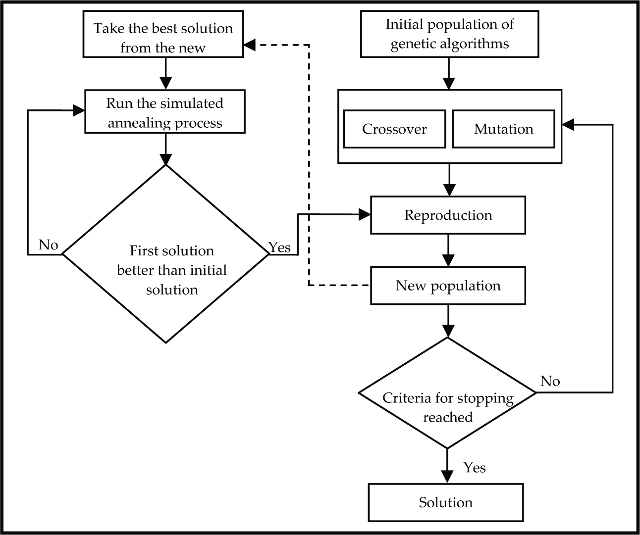
The proposed Hybrid Intelligent Solution System

6. Example problem

A parallel robot problem with 10 jobs and 3 parallel robots is considered below. The process times, delivery times and precedence constraints of the jobs were given. The solution, which minimizes mean tardiness, was obtained by considering this data. The problem was solved by using SPT (Shortest processing time), EDD (Earliest due date), FCFS (First come first served), CR (Critical ratio), SA, GA and a Hybrid Intelligent Solution System (GA+SA). The data and the results are given below. In Table 1, the jobs with process and due dates belonging to them are given. The precedence constraints of the jobs are given in Figure 6. In Table 2, the solutions obtained from the Hybrid System, GA, SA, SPT, EDD, FCFS and CR are given.

Table 1.

Processing time, due date and unequal release date of every job for the example problem

Job i	1	2	3	4	5	6	7	8	9	10
Processing time	3	2	8	5	2	7	4	9	1	5
Due date	2	1	3	4	5	3	8	4	2	6
Release date	2	3	4	1	6	3	2	5	4	3

Table 2.

The result of calculation for 10 × 3 problem size

Heuristic	Schedule	Mean Tardiness
SPT	M1: 2-5-7 M2: 1-4-8-10 M3: 3-6-9	15.6
EDD	M1: 2-6-8 M2: 1-4-7 M3: 3-5-9-10	14.8
FCFS	M1: 1-4-7-9 M2: 2-5-10 M3: 3-6-8	14.6
CR	M1: 3-6-8 M2: 2-1-4 M3: 5-7-9-10	15.4
GA	M1: 1-4-7-9 M2: 2-5-8-10 M3: 3-6	14.6
SA	M1: 2-6-8 M2: 1-4-7 M3: 3-5-9-10	14.8
HISS	M1: 1-4-7-9 M2: 2-5-8-10 M3: 3-6	14.6

Figure 6.

Precedence constraints of every job for example problem

7. Numerical experiment design

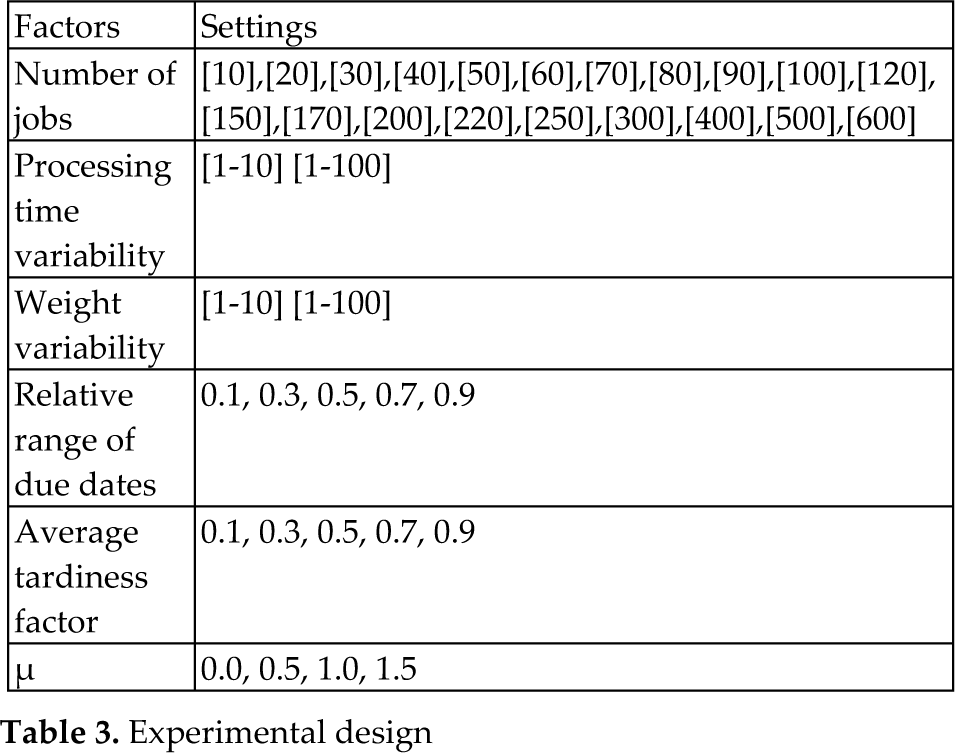
The number of jobs used in the problems in this study are given in Table 3. In this table, i denotes the jobs, and p_i is an integer: processing time and w_i is an integer: weight, which were generated from two uniform distributions. The functions of [1, 10] and [1, 100] are to create low or high variations, respectively. TF, which is the relative range of due dates, RDD and an average tardiness factor, were selected from the set [0.1, 0.3, 0.5, 0.7, 0.9]. Here, di is an integer: due date - from the uniform distribution [P (1-TF-RDD/2), [P(1-TF+RDD/2)] and it was generated for each job i. In these expressions, P denotes total processing time. Release dates are generated from a uniform distribution between 0 and μ∑pj. As summarized in Table 3, 80000 example sets were considered in total. All algorithms were coded in C++ and implemented on a Pentium IV 2.4 GHz computer during the implementation of algorithms.

Table 3.

Experimental design

Factors	Settings
Number of jobs	[10],[20],[30],[40],[50],[60],[70],[80],[90],[100],[120],[150],[170],[200],[220],[250],[300],[400],[500],[600]
Processing time variability	[1–10] [1–100]
Weight variability	[1–10] [1–100]
Relative range of due dates	0.1, 0.3, 0.5, 0.7, 0.9
Average tardiness factor	0.1, 0.3, 0.5, 0.7, 0.9
μ	0.0, 0.5, 1.0, 1.5

The problems were considered in 20 different sizes and for each size 400 different samples were examined. The parameters of the GA are given below. These parameters are first tried with different values, and according to the results of these experimental studies these parameters were determined as the best ones. In other studies, these parameters are determined in the same way as the ones obtained in this study. The optimal solutions obtained for different population sizes are given below in Figure 7 for the problem with dealing with the sizes 100 × 8. In Figure 9, the tardiness values for initial population and generations 100, 150 and 200 are presented. These figures give clear information about the selected parameters of GA.

Figure 7.

The obtained optimal solutions according to the different population sizes

Figure 8.

The effect of crossover rate to solution

Figure 9.

The obtained tardiness values for initial population and generations 50, 100 and 150

Population size : 25, Crossover rate :%100, Max generation : 150, Mutation rate :0.05.

As seen in Figure 7, to obtain an optimal solution, the different population size values were applied. When the population size is selected as 25, the optimal solution obtained is found to be better than ones examined with other population sizes. The population size does not affect the solution when it is higher than 25. This is because some of the results of the crossover and mutation processes are accepted as invalid solutions since they cannot give an appropriate order for precedence constraints during the running of GA. Therefore, the population size, which is higher than 25, does not affect the solution as significantly as shown in Figure 7 and furthermore it increases the process time. Additionally, the genetic algorithm was stopped once it had produced the same solution in 50 consecutive generations.

In Figure 8, the effect of crossover rate on the solution is shown. From the figure it can be clearly observed that when the crossover rate increases, better solutions can be obtained in better processing times.

In Figure 9, the tardiness values are given for the initial population, generation 50, generation 100 and generation 150. The graphic is created by using the best 25 chromosomes obtained from the initial population, generation 50, generation 100 and generation 150. As can be seen in the figure, a better population was obtained in generation 150.

8. Results and discussions

In this section the results are presented and evaluated based on the problems in different sizes for GA, SA and the designed GA+SA hybrid system.

The results show that GA gives better results than SA in large-size problems. In Table 4, the solutions obtained for different problem sizes are given. For each problem size, 100 different samples were used. GA and SA were applied to these samples. The average value of the obtained optimal solutions is revealed in the table. According to the average value, it can be clearly seen that GA gives the better result. In terms of CPU time, again it is GA that obtains a better result.

Table 4.

The results of the problems in different sizes

PROBLEM SIZE	Number of example	Average value of GA	Average Value of SA	CPU time for GA for an example	CPU time for SA for an example problem (s)	t statistics
10 × 2	100	31.24	24.84	4.32	6.12	4.47
20 × 3	100	72.59	81.32	5.76	8.43	6.32
30 × 5	100	84.86	112.78	17.42	24.55	8.75
40 × 6	100	114.83	140.84	24.53	36.49	11.65
50 × 7	100	162.36	181.63	32.77	52.87	11.94
60 × 8	100	175.75	229.74	41.61	71.67	11.42
70 × 7	100	214.48	268.39	54.94	83.90	12.82
80 × 8	100	253.83	338.68	75.39	99.13	15.38
90 × 8	100	313.92	398.26	90.28	121.19	16.78
100 × 8	100	395.45	512.35	110.33	143.66	18.36
120 × 8	100	459.98	548.48	140.14	178.42	19.87
150 × 8	100	547.49	579.85	174.21	191.29	22.93
170 × 8	100	600.29	736.47	241.33	130.79	22.42
200 × 8	100	785.93	978.88	260.89	279.89	24.06
220 × 8	100	847.26	1021.12	280.01	301.23	25.28
250 × 8	100	982.15	1245.37	312.73	356.47	30.86
300 × 8	100	1351.21	1889.28	379.42	403.88	32.55
400×10	100	1730.47	1987.33	410.53	443.76	35.49
500×10	100	2140.69	2378.56	447.27	481.56	37.38
600×10	100	2342.82	2602.51	478.29	198.55	37.92

In Table 5, the 100 samples given for each problem size are evaluated and the number of the results obtained by using GA which are better or equal to SA is shown. When we look at the results in Table 5, because of the structure of the selected problem, GA gave better results than SA especially for the small size problems; SA and GA gave the same solutions at a maximum rate of 21% and a minimum of % 2. However, GA mostly produced better results than SA in the implemented samples. On the other hand, when the problem size is equal to or larger than 90×8, GA gave better solutions then SA at a rate of 100% in the sample solutions. GA has shown itself to be successful for dealing with the large size problems. However, we cannot take this success of GA at dealing with the selected problem to apply too generally; in other words, we cannot simply say that GA is more successful then SA. According to the large t-test values for the average improvement, GA provides an important improvement and the amount of improvement is noteworthy at a confidence level of 99.5%.

Table 5.

Comparison of the results of the examples according to the optimal values

Problem size	Number of examples	Number of examples where GA is better than SA	Number of examples where GA is equal to SA
10 × 2	100	79	21
20 × 3	100	84	16
30 × 5	100	86	14
40 × 6	100	89	11
50 × 7	100	90	10
60 × 8	100	91	9
70 × 7	100	96	4
80 × 8	100	98	2
90 × 8	100	100	0
100 × 8	100	100	0
120 × 8	100	100	0
150 × 8	100	100	0
170 × 8	100	100	0
200 × 8	100	100	0
220 × 8	100	100	0
250 × 8	100	100	0
300 × 8	100	100	0
400×10	100	100	0
500×10	100	100	0
600×10	100	100	0
400×20	100	100	0
500×20	100	100	0
600×20	100	100	0

According to Figure 10, it is evident that the Hybrid Intelligent Solution System reaches the solution in a better process time and it can also find better solutions. In other words, adding SA to GA increased the performance of GA. GA and SA metaheuristics have some advantages compared to each other because of the algorithms which they use. Therefore, these two algorithms can be implemented in parallel and then they can share the best solution with each other to find a faster and better solution. It can clearly be seen in Fig. 10, that the hybrid solution system, which uses both algorithms together, gave better results compared to GA. The hybrid intelligent solution system reached the solution quicker. The hybrid solution system reached the final solution in approximately 50 generations whereas GA reached the final solution in about 92 generations. The hybrid system is more advantageous in terms of process time.

Figure 10.

Comparison of GA and Hybrid Intelligent Solution System

Since the hybrid system reaches the final solution when GA is still trying to reach the final solution, the hybrid system should be stopped from working at this point. In Fig. 10, the dotted line represents GA and the bold line represents the hybrid intelligent solution system.

It can clearly be seen in Table 6 that the hybrid system is more successful than GA. Additionally; the hybrid system is also successful when it comes to the process time, as seen in the table. According to the large t-test values it is evident that hybrid system is more successful than GA at a level of 99.5 %. In Table 7, the number of solutions that are better obtained by using the hybrid system than GA are given. In Table 7, it can be seen that GA and SA played a significant role in increasing their own success in the hybrid intelligent solution system. Especially, as seen in Table 7 the performance of GA has been increased by the hybrid system and more successful solutions have been found.

Table 6.

Comparison of Hybrid Intelligent Solution System and GA for different problem sizes

PROBLEM SIZE	Number of example	Average value of GA	Average Value of GA+SA	CPU time for GA for an example (s)	CPU time for GA+SA for an example (s)	t statistics
10 × 2	100	31.24	29.38	4.32	3.41	2.00
20 × 3	100	72.59	70.64	5.76	5.12	2.00
30 × 5	100	84.86	79.21	17.42	11.46	2.05
40 × 6	100	114.83	101.29	24.53	18.49	2.06
50 × 7	100	162.36	150.36	32.77	28.74	2.42
60 × 8	100	175.75	163.27	41.61	36.54	2.43
70 × 7	100	214.48	201.87	54.94	47.62	2.43
80 × 8	100	253.83	239.39	75.39	66.45	2.44
90 × 8	100	313.92	289.47	90.28	80.17	2.44
100 × 8	100	395.45	374.56	110.33	90.34	2.49
120 × 8	100	459.98	432.46	140.14	112.05	2.51
150 × 8	100	547.49	512.73	174.21	155.39	2.59
170 × 8	100	600.29	563.75	241.33	232.27	2.69
200 × 8	100	785.93	752.45	260.89	239.83	3.24
220 × 8	100	847.26	804.55	280.01	259.01	3.78
250 × 8	100	982.15	933.49	312.73	389.36	3.85
300 × 8	100	1351.21	1285.17	379.42	360.22	4.02
400×10	100	1730.47	1683.42	410,53	386.45	5.84
500×10	100	2140.69	2002.08	447,27	411.03	6.74
600×10	100	2342.82	2241.14	478,29	453.27	7.92

Table 7.

Comparison of Hybrid System and GA according to optimal values

Problem size	Number of examples	Number of examples where the Hybrid System is better than GA	Number of examples where GA is equal to the Hybrid System
10 × 2	100	8	92
20 × 3	100	9	91
30 × 5	100	10	90
40 × 6	100	12	88
50 × 7	100	13	87
60 × 8	100	14	86
70 × 7	100	14	86
80 × 8	100	16	84
90 × 8	100	16	84
100 × 8	100	18	82
120 × 8	100	19	81
150 × 8	100	21	79
170 × 8	100	21	79
200 × 8	100	22	78
220 × 8	100	23	77
250 × 8	100	25	75
300 × 8	100	27	73
400×10	100	29	71
500×10	100	30	70
600×10	100	32	68
400×20	100	32	68
500×20	100	32	68
600×20	100	33	67

9. Conclusions

In this paper a Hybrid Intelligent Solution System (HISS) based on using GA and SA has been proposed to solve parallel robot scheduling to minimize mean tardiness with unequal release date and precedence constraints. A Simulated Annealing (SA) process is used to support the Genetic Algorithms (GA). GA, SA and HISS have been applied to different sizes of parallel robot problems. During the study, it is observed that because of the structure of the selected problems GA mostly gave better results than SA and GA has shown its success especially when dealing with the big size problems. However, GA's success in dealing with the selected problem in this study cannot be generalized. On the other hand, the Hybrid Intelligent Solution System reached the solution in a better process time and it also found better solutions. This means that adding SA to GA increased the performance of GA.

In conclusion, the results show that the proposed HISS outperforms GA in effectiveness (the quality of the solution) and efficiency (less computational time). In the future, this proposed HISS could be applied to non-identical parallel robots.

References

Çakar

Yazgan

Köker

(2008) Parallel Manipulators, New Developments. I-Tech Education and Publishing, Vienna, Austria: 153–170.

Köker

Ferikoglu

(2001) Development of a vision based object classification system for an industrial robotic manipulator. 8th IEEE International Conference on Electronics, Circuits and Systems, Vol.3, Malta: 1281–1284.

Tsuchiya

(2007) Scheduling optimization of component mounting in printed circuit board assembly by prioritizing simultaneous pickup. International Conf. on Intelligent Robots and Systems, San Diego, CA: 2913–2918.

Picard

J-C

Queyranne

(1977) On the integer-valued variables in the linear vertex packing problem. Mathematical Programming 12(1):97–101.

Graves

(1981) A review of production scheduling. Operations Research 29(4):646–675.

Allahverdi

Gupta

JND

Aldowaisan

(1999) A review of scheduling research involving setup considerations. Omega 27(2):219–239.

Mokotoff

(2001) Parallel machine scheduling problems: A survey. Asia-Pacific, Journal of Operational Research 18(2):193–242.

Asano

Ohta

(2002) A heuristic for job shop scheduling to minimize total weighted tardiness. Computers and Industrial Engineering 42(2–4):137–147.

Brucker

Knust

Schoo

Thiele

(1998) A branch and bound algorithm for the resource-constrained project scheduling problem. European Journal of Operational Research 107(2):272–288.

10.

Dunstall

Wirth

(2005) Heuristic methods for the identical parallel machine flow time problem with set-up times. Computers and Operations Research 32(9):2479–2491.

11.

Kurz

Askin

(2001) Heuristic scheduling of parallel machines with sequence dependent set-up times. International Journal of Production Research 39(16):3747–3769.

12.

Lin

(2004) Parallel machine scheduling of machine-dependent jobs with unit length. European Journal of Operational Research 156(1):261–266.

13.

Kim

Bobrowski

(1997) Scheduling jobs with uncertain setup times and sequence dependency. Omega 25(4):437–447.

14.

Kim

Jane

Chen

(2002) Unrelated parallel machine scheduling with setup times using simulated annealing. Robotics and Computer Integrated Manufacturing 18(3–4):223–231.

15.

Kim

Chen

(2003) Unrelated parallel machine scheduling with setup times and a total weighted tardiness objective. Robotics and Computer Integrated Manufacturing 19(1–2):173–181.

16.

Glass

Potts

Shade

(1994) Unrelated parallel machine scheduling using local search. Mathematical and Computer Modelling 20(2):41–52.

17.

Yang

(2011) Heuristic Algorithms for Scheduling on Uniform Parallel Machines with Head and Tail. Journal of Systems Engineering and Electronics 22(3):462–467.

18.

Jouglet

Savourey

(2011) Dominance Rule For The Parallel Machine Total Weighted Tardiness Scheduling Problem with release dates. Computers & Operations Research 38(9):1259–1266.

19.

Saricicek

Celik

(2011) Two-meta Heuristics for parallel machine scheduling with job splitting to minimize total tardiness. Applied Mathematical Modelling 35(8):4117–4126.

20.

Vallada

Ruiz

(2011) Genetic Algorithm For The Unrelated Parallel Machine Scheduling Problem With Sequence Dependent Setup Times. European Journal Of Operation Research 211(3):612–622.

21.

Lin

Pfund

Fowler

(2011) Heuristics For Minimizing Regular Performance Measures in Unrelated Parallel Machine Scheduling Problem. Computers & Operations Research 38(6):901–916.

22.

Balin

(2011) Non-identical Parallel Machine Scheduling Using Genetic Algorithm. Expert Systems with Applications 38(6):6814–6821.

23.

Lin

Ying

(2011) Minimization of Total Tardiness on Unrelated parallel machines with sequence and machine dependent setup times under due date constraints. International Journal of Advanced Manufacturing Technology 53(1–4):353–361.

24.

Yang

(2011) A simulated Annealing Approach to minimize the maximum Lateness on Uniform Parallel Machines. Mathematical and Computer Modelling 53(5–6):854–860.

25.

Chang

Chen

(2011) Integrating Dominance Properties With Genetic Algorithms For Parallel Machine Scheduling Problems With Setup Time. Applied Soft Computing 11(1):1263–1274.

26.

Toksari

Guner

(2010) Parallel Machine Scheduling Problem to minimize the earliness/tardiness costs with Learning effect and Deteriorating jobs. Journal of Intelligent Manufacturing 21(6):843–851.

27.

Biskup

Hermann

Gupta

JND

(2008), Scheduling Identical Parallel Machines to Minimize Total Tardiness. International Journal of Production Economics 115(1):134–142.

28.

Zhou

Zheng

Wang

(2007) Genetic Algorithm-based minimization of weighted completion time of parallel multi-machine Scheduling. Proceeding International Conference of Industrial Engineering and Engineering Management, 91–95.

29.

Gomez-Gasquet

Franco-Preyra

Navarro-Varela

. An experimental Investigation on Relegated Parallel. Proceeding of the second International Conference on Operations and Supply Chain Management.

30.

Liaw

Lin

Chen

(2003) Scheduling unrelated parallel machines to minimize total weighted tardiness. Computers & Operations Research 30(12):1777–1789.

31.

Missbauer

(1997) Order release and sequence-dependent setup times. International Journal of Production Economics 49(2):131–143.

32.

Srivastava

(1998) An effective heuristic for minimizing makespan on unrelated parallel machines. Journal of the Operational Research Society 49(8):886–894.

33.

Martello

Soumis

Toth

(1997) Exact and approximation algorithms for Makespan minimization on unrelated parallel machines, Discrete Applied Mathematics 75 (2): 169–188.

34.

Chen

Z-L

Powell

(1999) Solving parallel machine scheduling problems by column generation. INFORMS Journal on Computing 11(1):78–94.

35.

Salem

Anagnostopoulos

Rabadi

(2000) A branch-and-bound algorithm for parallel machine scheduling problems. In: Society for computer simulation international (SCS). Portofino, Italy.

36.

Néron

Tercinet

Sourd

(2008) Search tree based approaches for parallel machine scheduling. Computers and Operations Research 35(4):1127–1137.

37.

Baev

Meleis

Eichenberger

(2002) An experimental study of algorithms for weighted completion time scheduling. Algorithmica 22:34–51.

38.

Van den Akker

Hoogeven

Kempen

(2005) Parallel machine scheduling through column generation: minimax objective functions, release dates, deadlines and/or generalized precedence constraints. Technical Report, Utrecht University

39.

Kasahara

Narita

(1985) Parallel processing of robot arm control computation on a multimicroprocessor system. IEEE J. of Robotics Automation RA-1(2):104–113.

40.

Chen

Lee

CSG

Hou

ESH

(1988) Efficient scheduling Algorithm algorithms for robot inverse dynamics computation on a multiprocessor system. IEEE Transaction on Systems, Man and Cybernetics 18:729–743.

41.

Chang

Y-L

(1991) Heuristics for minimizing mean tardiness for m parallel machines. Naval Research Logistics 38:367–381.

42.

Wilkerson

Irwin

(1971) An improved algorithm for scheduling independent jobs. AIIE Transactions 3:239–245.

43.

Çakar

Köker

Demir

(2008) Parallel Robot Scheduling To minimize Mean Tardiness With Precedence Constraints Using A Genetic Algorithm. Advance in Engineering Software 39:47–54.

44.

Kanjo

Ase

(2003) Robust scheduling in a multi robot welding system. Transaction of the Institute of systems, Control and Information Engineers 16(8):369–376.

45.

Jun

Ying

(2002) A genetic algorithm based approach to intelligent optimization for scheduling dual resources with robots. Robot 24(4):342–357.

46.

Zacharia

Asparagathos

(2005) Optimal robot task scheduling based on genetic algorithms. Robotics and Computer Integrated Manufacturing 21(1):67–79.

Parallel Robot Scheduling to Minimize Mean Tardiness with Unequal Release Date and Precedence Constraints Using a Hybrid Intelligent System

Abstract

Keywords

1. Introduction

2. Formulation of the objective function

3. Genetic algorithms

3.1 Modelling of the problem using Genetic Algorithms

3.2 Preparing Initial Population

3.3 Crossover

3.4 Mutation

3.5 Reproduction

4. Simulated annealing

4.1 Simulated annealing algorithm

5. Proposed hybrid intelligent solution system

6. Example problem

7. Numerical experiment design

8. Results and discussions

9. Conclusions

References