Sage Journals: Discover world-class research

Abstract

The concept of an algorithm developed for the segmentation of a road border from the content of an image produced by a forward looking TV camera mounted on a moving vehicle is presented in this paper. The extraction of a road boundary is an important step in the context of autonomous vehicle guidance, enabling further calculations of distance from the border, direction of a road, etc. The main idea behind this approach is that the texture of a road is different enough in comparison to the textures characterizing the surrounding environment, allowing the separation of the overall image into a few distinguishable regions. The segmentation algorithm combines the texture descriptors of a statistical nature and the ones based on a grey level co-occurrence matrix. The significance of this work is mainly in the practical verification of the proposed algorithm and in the testing of the real limits of its application.

Keywords

Autonomous vehicles Digital image processing Image segmentation Texture Texture classification

1. Introduction

The field of autonomous guidance of ground vehicles (wheeled robots, cars etc.) has rapidly developed during the last two decades. The possible applications span from cases where the vehicle moves autonomously along very well arranged highways with a number of distinguishable landmarks around, up to cases where the object moves through a completely unknown environment, along a road/path hardly separable from the local background. As a reasonable step toward fully autonomous guidance, a number of applications that have the nature of a “driving assistant” are envisaged. A number of heterogeneous sensors and systems are used in the context of “intelligent transportation systems”. The forward looking TV camera is one of the most popular and useful ones. The digitized image coming from the camera is a source of valuable information related to the task of recognition of a road/lane and its borders, detection of other subjects/obstacles on the road (e.g., other vehicles, pedestrians), detection and recognition of traffic signs, lights, etc. We have limited our attention here toward the task of the separation of the road region, or more precisely, the extraction of the border between the road and the surrounding background. This part of the image is important in order to calculate the vehicle's distance from the border, to estimate the radius of a road's curvature, as well as to estimate the heading and slope of a road (in cooperation with some other inertial or magnetic instruments, or prior known data).

The inspiration for this research has been found in some of relevant works referenced in Section 7. The scope of methods used in the computer vision for the control of intelligent road vehicles is given in [1], while a more general survey of the usage of vision for autonomous guidance was done in [2] and specifically for the purposes of mobile robot navigation, in [3]. The fundamentals of image segmentation, texture based descriptors and of basic pattern recognition relevant to the image processing applications are given in textbooks [4 –6]. Articles [7 –12] discuss the task of road border extraction using different methods (optical flow measurements, edge detection followed by Hough transform, segmentation based on colour contents, colour feature combined with line and road following, texture description alone and texture combined with colour). In [13 –15], for the same task, the focus is shifted more towards proper road modelling (the border is modelled as a straight or parabolic line, both for indoor and outdoor applications, or lines are detected in pairs, which is typical for an urban traffic environment). In papers [16–17] the authors go further by including additional devices like odometers or inertial instruments, in order to combine the information supplied by them with the visual tracking process and to provide final information about the vehicle's position/velocity on the road. Articles [18–19] are referenced here basically as examples of road segmentation algorithms oriented toward real-time applications. Description of textures and their classification was of particular interest in this paper. The authors of papers [20 –23] have discussed this problem of different aspects relevant to our approach (how to reduce the time for recognizing the texture as one out of predefined set, how to make the acquisition over multiple windows of different size, how to find the subset of relevant features that are sufficient to capture the important properties of the set of classes that are to be distinguished and how to make so called pixel-based texture classification which determines the class that every pixel of an input image belongs to). Finally, articles [24 –27] are oriented toward combinations of the usage of texture descriptors based on a co-occurrence matrix and other features like colour and variance, as well as classifications based on combinations of light intensity and colour with texture.

Generally, if one wants to extract the border between two or more regions in an image representing the scene in front of a vehicle, (the road being one of them) there are two basic approaches:

Edge Detection. Borders between the regions are characterized by appreciable light intensity variations and in order to extract these pixels some previous high pass filtration is preferable, after which the appropriate segmentation procedure separates the points where the gradient values are above the specified level (threshold).

Region Detection. The region of road can be characterized using the range of values of some descriptor(s), such that the other regions around are well distinguishable from the road and the road border is extractable this way. These descriptors can be related to the light intensity, colour, or different descriptions of a texture.

The use of texture descriptors is suggested in this paper for the defined type of task. One type of these descriptors (statistical ones) are related to the light intensity content typical for some parts of the road image and are generally based on statistical moments calculated for the population of pixels belonging to them (histogram moments). The other types relevant for this approach are based on a light intensity co-occurrence matrix and introduce the information about spatial relationships between pixels with different light intensities inside the road area.

None of these descriptors seems universally applicable for all types of roads and local backgrounds. Our idea is to make the segmentation algorithm semiautomatic, meaning that the simple initial acquisition of data is made by a human operator (driver), while the remaining procedure is fully automatic. As the first part of this procedure, the choice of the best candidates among descriptors of both types is done. The threshold values between classes (road, near background, far background, etc..) are found by minimization of erroneous classification. The classification is extended to two dimensions in order to obtain a balance between statistical and spatial texture characteristics, due to the fact that none of the regions are fully uniform regarding any descriptor. As a result of the intention that the algorithm should finally work in real time, very precise calculation of all points belonging to the border (pixel-based texture classification) is avoided. Instead, an initial scanning with a window of 64×64 pixels is followed by the appropriate splitting of the windows to 32×32 and 16×16, around the rudimentary estimated border (coarse to fine segmentation). Appropriate morphological filtration based on the assumption that the road region should be connected is the next step, while the whole procedure for one frame is finished by polynomial fitting through the “stairs-like” border segmented up to this point.

The novelty of the approach presented here mainly consists of the following aspects:

The automatic choice of the best candidates for descriptors – the most suitable ones for the actual scene

An easy way of introducing basic training via acquisition of statistical information related to descriptor values.

Fast threshold specification via reduction of the multidimensional classification task to one-dimension.

A “low-resolution” approach in a splitting/merging type of image segmentation.

The scope of the texture descriptors used here and the reasons why such an initial choice was made are explained in Section 2. The constituent steps of the segmentation algorithm are described in Section 3. The segmentation algorithm is initially verified through all these steps using one typical road image in Section 4. Some other typical cases are shown in Section 5 to point out the algorithm limits and some possible steps in order to overcome these problems. Finally, the overall conclusions and directions for further work related to the processing of the sequence (frame-by-frame prediction of a border location, adaptation of algorithm parameters) are given in Section 6.

2. Texture Descriptors

Texture can be observed in the repetitive structural patterns of surfaces of both natural and artificial objects and may intuitively be viewed as a measure of surface properties such as smoothness, coarseness, regularity, etc. [22]. There are a number of ways to characterize texture. Typical examples are statistical, structural and spectral approaches, although a strict formal approach or precise definition of texture is not available. Two of main application domains related to texture-based image analysis are: 1) supervised texture classification (determining the class (texture) to which an image or image region belongs, using a set of examples for each class as a training set) and 2) unsupervised texture segmentation (partitioning of a given image into disjoint regions of uniform texture). The approach used in this paper is a mixture of these two. While the main task consists of the partitioning of an image into uniform regions not known in advance, the starting point in the segmentation algorithm has the nature of a simple training process.

Among the statistical descriptors, the following have been considered, inside the image region of dimensions N * N pixels of light intensities z_i in the range from l_min = 0 to l_max = L − 1 = 255, with individual probability of occurrence, p(z_i) as estimated from the histogram. Standard deviation of light intensities:

\begin{array}{l} σ = \sqrt{μ_{2} (z)} = \sqrt{\sum_{i = 0}^{L - 1} {(z_{i} - m)}^{2} p (z_{i})}, \\ m = \sum_{i = 0}^{L - 1} z_{i} p (z_{i}) \end{array}

(1)

Third moment:

μ_{3} (z) = \sum_{i = 0}^{L - 1} {(z_{i} - m)}^{3} p (z_{i})

(2)

Uniformity:

u = \sum_{i = 0}^{L - 1} p^{2} (z_{i})

(3)

Average entropy:

e = - \sum_{i = 0}^{L - 1} p (z_{i}) {log}_{2} p (z_{i}) p \in [0, 1]

(4)

The structural descriptors considered in this paper are derived from a so called “light intensity co-occurrence matrix”, representing spatial relationships between pixels of different light intensities. Any element of this matrix C_ij (of dimensions 256×256) means the number of occurrences when a pixel with light intensity j is located at a particular position relative to the observed pixel with light intensity i (e.g. northern neighbor).

The following descriptors are defined:

Contrast:

C = \sum_{i} \sum_{j} {(\frac{i - j}{N})}^{2} c_{i j} / \sum_{i} \sum_{j} c_{i j} ​ ​

(5)

Inverse moment of first order:

I M = \sum_{i} \sum_{j} c_{i j} / {(i - j)}^{k} i \neq j ​ ​, k = 1

(6)

Uniformity:

U = \sum_{i} \sum_{j} c_{i j}^{2} ​_{​}

(7)

Entropy:

E = - \sum_{i} \sum_{j} c_{i j} \log_{2} c_{i j}

(8)

Although none of these descriptors can be universally applicable for a specified task and none of the image regions can be considered as completely uniform, this approach tends to find which among them (in both categories) can be adopted as the best representative in each particular case. Simultaneous consideration of both statistical and structural properties has been used as a measure of redundancy and tries to take into account not just global statistical measures of coarseness, but also some structural regularities of the road region distinguishing it from other parts of image.

3. Segmentation Algorithm

A very basic assumption is that the whole image generally consists of three distinguishable regions: road, local (near) background and far background. The very first step in this procedure is done by a human operator (driver), just by pointing to three different points on image that best represent these three classes.. The image shown in Fig. 1 [28] represents the typical content of the scene in front of the forward looking camera mounted on the vehicle moving along the empty road. Square inspect windows of dimension 64×64 are automatically generated around these points.

Figure 1.

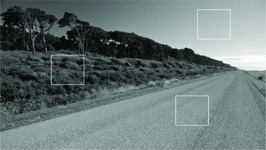
Test image with three inspect windows.

All eight descriptors mentioned above are calculated for the populations of the pixels inside these inspect windows. It is a reasonable assumption that the texture of the near background is generally less homogeneous (coarser) than the one representing the road, while the texture of the far background (especially because of the sky) is more homogeneous (smoother).

Grey level histograms and co-occurrence matrices (represented as images) for all three inspect windows are shown in Fig. 2.

Figure 2.

Grey level histograms and co-occurrence matrices for road (a, b), background (c, d) and sky (e, f) .

There are obvious differences between the types of histograms shown in Fig. 2 (a, c, e) as well as in the case of the co-occurrence matrices shown in Fig 2. (b, d, f). According to them, one can expect that the descriptors listed above are going to take numerical values allowing the separation of the image regions. It is important to notice that the proper choice of positions of inspect windows is of high importance for the whole process of segmentation.

The border segmentation algorithm consists from the following seven steps:

The Choice of the Best Candidate among Descriptors

In order to obtain good separation of classes, the values of the descriptors specified via equations (1 – 8) inside inspect windows should be as different as possible. High ratios between the values of texture descriptors inside three regions are preferable (both ratios between maximum and medium values and medium and minimum values, among these three). The criterion for the choice of the best candidate adopted here searches for the maximal average of these two ratios (Max {Avg [max/med, med/min]}), while any one of them should not be less than 1.5. If inside one type of descriptors there are no ratios greater than 1.5, new pointing should be done, because otherwise the class separation would be strongly affected. As a result of this step, the proper candidates are selected to be applied in further segmentation processes.

Acquisition of Relevant Data

In spite of the fact that the inspect windows are located in the representative positions, only one value of descriptor per class cannot be a good representation of the whole class. In order to acquire some statistically relevant information, the next step consists of the calculation of the values of two selected descriptors over the set of windows around the initial one. The initial square is shifted in all four main directions for 16 pixels, pixel by pixel, producing 1024 values of the two selected descriptors per each class. This step has the nature of a simple training procedure. The set of 1024 values carry the information about how the particular descriptor is distributed over all three areas. Because of the fact that this acquisition phase could be time consuming, the mechanization of appropriate calculations of statistical moments and co-occurrence matrices given in Section 2 are made as iterative ones. For any new translated position of the window, the result obtained for the previous one is corrected by the amounts related to disappearing and newly added rows/columns.

The actual distributions of descriptor values inside the areas encompassed by these 1024 windows can be pretty different. Sometimes the distribution is not symmetrical around the mean value, or it could be even bimodal if the whole area around the inspect window encompasses two textures that are “different enough”. The last case is most frequent in the near background class, although it can be obtained for the sky (clear/cloudy) and for non-uniform road texture also. After the mean values and standard deviations are calculated for both descriptors and all three classes, the assumption that the values of the descriptors are normally distributed is adopted. A number of experiments have verified that this approximation can be used in order to specify the threshold value (or the separation line between classes) and was acceptable even if the actual distributions have not been Gaussian ones. Segmentation based on the identification of particular probability density functions would be a more adequate method, but both the identification phase itself as well as the more complex method of the calculation of separating points/lines would result in a meaningful consumption of computing time.

Definition of a Threshold

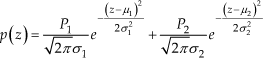
If the classification is to be done according to one texture descriptor, the threshold values separating the classes are to be defined. The simplest idea is to specify them in the middle of the distance between the prototype values of descriptors (either directly from inspect windows or based on calculated mean values). However, it was realized in practice that due to the non-uniform nature of all three regions, the information about the standard deviation of a particular feature should also be used, rather than using simple Euclidean distance. As a result of this, the threshold values are set at the points where the probability of membership of both neighboring classes is equal (at the intersections of particular probability density functions). Assuming that the partial probability density functions are of Gaussian type, the overall probability density function can be represented as their mixture:

p (z) = \frac{P_{1}}{\sqrt{2 π} σ_{1}} e^{- \frac{{(z - μ_{1})}^{2}}{2 σ_{1}^{2}}} + \frac{P_{2}}{\sqrt{2 π} σ_{2}} e^{- \frac{{(z - μ_{2})}^{2}}{2 σ_{2}^{2}}}

(9)

While the required threshold value can be found by solving binomial equation:

A T^{2} + B T + C = 0

(10)

where:

\begin{array}{l} A = σ_{1}^{2} - σ_{2}^{2} \\ B = 2 (μ_{1} σ_{2}^{2} - μ_{2} σ_{1}^{2}) \\ C = σ_{1}^{2} μ_{2}^{2} - σ_{2}^{2} μ_{1}^{2} + 2 σ_{1}^{2} σ_{2}^{2} \ln (σ_{2} P_{1} / σ_{1} P_{2}) \end{array}

σ_i – standard deviation of class i, i = 1,2

μ_i – mean value of class i, i = 1,2

P₁ = P₂, a priori probability of occurrence of both classes.

The value which lies in between two mean values is chosen from two solutions of equation (10). The formal application of this approach sometimes does not guarantee acceptable results. Therefore we introduced the following exceptions:

If both standard deviations are much less than half the distance between two mean values, the threshold is adopted in the middle of the two mean values.

If just one of the standard deviations is much less than the half-distance, while the other one is comparable with it, the threshold value is shifted toward the class characterized by the small value of standard deviation (one quarter of distance between mean values, relative to the mid-point).

If at least one standard deviation is higher than the distance between mean values it is an implicit sign that the distribution(s) are not Gaussian and the threshold is adopted at the middle point again. Otherwise, for example, the solutions of (10) could be completely outside the range defined between two mean values.

Only if both standard deviations are comparable to the half-distance between mean values, should the solution of eq. (10) be used as a threshold value.

The choice of the threshold value of a particular descriptor that is separating two classes (regions) is calculated in this way, according to the actual distributions of the descriptor values (only if they are really normal ones). If the classes are very well separated, the Euclidean distance is also applicable. The flowchart shown in Figure 3 is an illustration of the above mentioned specification of the threshold value (T), discriminating between two classes represented via their mean values (M1 and M2) on the distance d.

Figure 3.

Flowchart illustrating the specification of the threshold value of descriptor.

Extension to Two Dimensions

As was mentioned in Section 2, none of the texture descriptors can be assumed as something uniquely characterizing the whole region of interest. In order to balance the statistical information provided by the best descriptor from the first group and the spatial information introduced by the best descriptor from the second one, the classification is finally done in two-dimensional descriptor space. Separating curves can be defined as the straight lines (based on Euclidean distance from the prototype points – defined as the appropriate pair of mean values) or as the projections of the curves obtained at the intersections of two dimensional probability density functions (the typical 3D representation of distributions of values of two descriptors for three classes is represented in Fig. 4) In order to overcome numerical problems arising from the fact that ranges of candidate descriptors could be extremely different, a normalization procedure has been performed in a way that all absolute values of one type of descriptor (including mean values and standard deviations) are divided among three classes by the maximal mean value of that particular descriptor. The descriptor plane is now approximately reduced to a unity square (still allowing some values outside 0–1 range). Two-dimensional distributions around the normalized mean values have generally elliptic profiles. 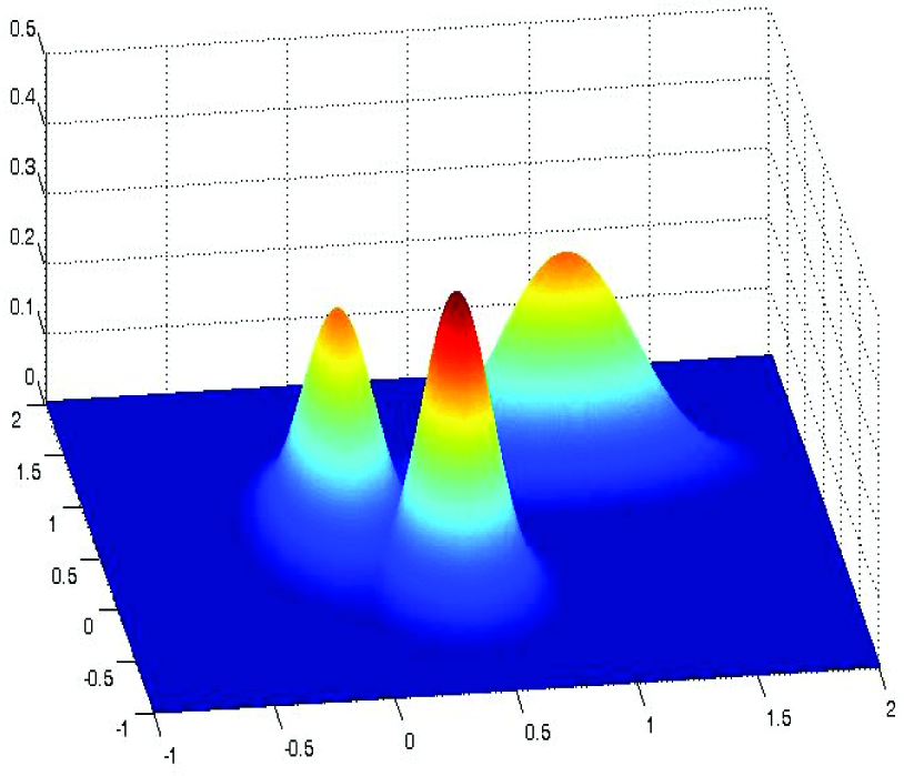The same reasoning in threshold specification described above in the one-dimensional case is now applied along the line connecting two particular normalized mean values (Road-Sky and Road-Background). Equivalent standard deviations (σ_RS, σ_SR, σ_RB, σ_BR) are calculated for the particular direction, based on standard deviations partially known for both descriptors. The point defined this way determines the crossing of the discriminating straight line, perpendicular to the line connecting mean values (see Fig. 5)

Figure 4.

Typical distributions of two normalized values of texture descriptors for three specified classes.

Figure 5.

The example of discriminating lines extracting the road class in two-dimensional case.

Merging/Splitting procedure

The initial segmentation is made after scanning the image by the 64×64 pixels winow, starting from the top-left position and classifying every window to the appropriate class according to thresholds/discriminating curves specified above. As a result of this first pass, one obtains an image of very poor resolution, just showing the rudimentary areas belonging to three mentioned classes.

The next step consists of the gradual splitting of those windows that are found to be on both sides of the road border. This splitting is done in two steps, down to the 32×32 and 16×16 pixel windows. It was found that this way of merging/splitting will reduce the overall computation time in comparison to the initial scanning with the 16*16 window over the whole image. Moreover, further splitting of the window would lead to a refined border, but on the other hand, further reducing of the size of the window would deteriorate the statistical validity of data. Finally, the other extreme consisting of scanning with the 64*64 window (statistically preferable) over the whole image, pixel-by-pixel, produces typical “over-segmentation” results, i.e., the border is “too precisely” extracted (too much dependence on local variations around the border) and there is a need for a lot of morphological processing after.

Morphological Filtration

Some morphological filtration is needed even after the previous step produced the segmented image of reduced spatial resolution. Before the road border is finally extracted, one should eliminate all portions of the image classified as the road that are not connected to the “main body” of the road, as well as filling the holes over the road area (either due to shadows/reflections or due to the existence of other vehicles).

During the first two passes (using the 64×64 and 32×32 windows), only an elimination of non-connected regions has been used. After the final splitting to the 16×16 pixel size, the final morphological process is made using the opening (erosion followed by dilation), with a 17×17 square structuring element, finally followed by an erosion with a 3×3 square structuring element.

Border Fitting

After all the previous steps, the road border is extracted as a stairs-like set of points. It is now possible to make the appropriate fitting through them. For the purpose of estimating the distance from the border and the road orientation (finding the vanishing point based on left and right borders) it is appropriate to fit a line through the set(s).

According to the type of morphological processing that was used, the set of most informative points along the stairs consisted of:

the “leftmost on each stair on the ascending part” and

the “rightmost on each stair on the descending part”.

If one is interested in more sophisticated results (i.e., positioning of the vehicle on a map, vehicle's speed control according to the actual road curvature, etc.) some type of polynomial approximation through the complete set of points is needed (most frequently, binomial).

All these steps are illustrated in the next Section, using the test image given in Fig. 1.

4. Verification of the Algorithm

The values of the specified descriptors for the position of inspect windows as in Fig. 1. are given in the following tables. The best candidate column is shaded:

Table 1.

Representative values and relative ratios (statistical descriptors)

	σ	μ₃	u	e
road	7.7272	127.6424	0.0396	4.9601
ground	27.7027	11036.3776	0.0111	6.7244
sky	8.9209	35.4436	0.0307	5.1242
max/med	3.1054	86.4632	1.2893	1.3123
med/min	1.1545	3.6013	2.7681	1.0331
avg	2.1299	45.0323	2.0287	1.1727

As one can see, the average entropy for example, is not at all appropriate to be used as a descriptor due to the narrow range of representative values for all three regions. Actually, the third moment is the only statistical descriptor where the ratio between any two region representative values is at least greater than 1.5.

Similarly, like in the case of statistical descriptors, one can recognize that contrast and inverse moment of first order can be preferable candidates for region classification, while uniformity is still a good descriptor, in comparison to entropy specified in structural context.

Table 2.

Representative values and relative ratios (structural descriptors)

	C	IM	U	E
road	0.0013	0.1568	0.0026	9.1156
ground	0.0126	0.0033	0.0005	11.2361
sky	1e-8	0.3986	0.0156	6.1867
max/med	9.6995	2.5421	5.9115	1.2326
med/min	104.5788	47.8462	5.4592	1.4734
avg	57.1391	25.1941	5.6853	1.353

In order to acquire valid statistical information, the initial square of size 64×64 is shifted in all four main directions for 16 pixels, pixel by pixel, producing 1024 values of selected descriptors per class. The following are results (mean values and standard deviations) obtained for a statistical descriptor (third moment), for three different window sizes (64×64, 32×32, and 16×16):

Table 3.

Statistical parameters of distribution of third moment values for different window sizes

	m _64x64	σ_{64x 64}	m _32x32	σ_32x32	m _16x16	σ_{16 x16}
road	192.4	176.5	123.8	106.5	37.9	28.8
gnd	10687	1021	14989	3014	9954	7447
sky	41.55	18.86	4.99	3.36	1.27	1.06

Threshold values discriminating between the classes in the case of the 64×64 window are obtained numerically as t₁ = 82.21 and t₂ = 1768.9. Graphical interpretation of threshold t₁ separating the road region from sky region is given in Fig. 6.

Figure 6.

Distributions of third moment values.

Fig. 7 illustrates the segmentation results when only the third moment is used (one dimensional case). Sub-figures a) sky, b) background and c) road show the results of crude segmentation for all three classes, while the result given in d) is obtained for the road class, after the removal of disconnected regions and all subsequent splitting and morphological filtration steps. Intermediate results obtained during the road region extraction in two-dimensional case are shown in Fig. 8. The very final extraction of road-ground borders is now illustrated after the appropriate line fitting, using the lines' intensification in white.

Figure 7.

Segmentation results obtained using the third moment as descriptor.

Figure 8.

Intermediate results during the road region extraction (two-dimensional case): a) after primary scanning; b) after elimination of disconnected regions; c) after final splitting; d) after final morphological processing and line fitting

5. Algorithm Performances and Limits

There are a number of principal problems to be mentioned as algorithm limits, in order to discuss what other criteria and reasoning should be included as a kind of algorithm upgrade.

Fig. 9.a illustrates typical problems related to two facts:

Figure 9.

The example of a scene where just the lower part of image is informative. Extracted borders are intensified in white.

The area of sky is not wide enough to provide placing of a set of 64×64 windows;

There is a slope of the road visible in the upper part of the image and the further part of the road is undistinguishable from the background. The result given in Fig. 8.b is obtained after initial placing of a 32×32 window and subsequent splitting down to 8×8 pixel size.

The main conclusions that can be derived from this example are:

Sometimes it is not relevant to have more than two classes. Classification of “road”, “non-road” regions can be acceptable.

This is true especially if attention is paid to the lower part of the image dominantly (there is no contact between the road and further background).

The following is an example where the road area includes visible lane borders. If some kind of gradient algorithm had been used, the detection of a lane border might be easier in these cases. On the contrary, if the region texture is used for description, the existence of visible lane borders makes this task a little bit harder – declaring by texture that the white lane borders are different from the road itself. The result shown in Fig. 10 illustrates this type of road environment. One can conclude that the border lines detected by this algorithm would tend to be a little bit inside the road region relative to the actual ones.

Figure 10.

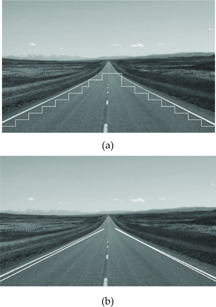
The example of a scene where the lane borders are visible: a) result of 2D classification, b) final border fitting.

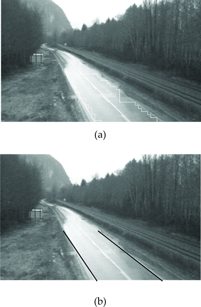
The existence of visible white lines separating the tracks in a typical highway environment can generally produce these problems because the texture is different enough in comparison to the typical road texture. Sometimes, as in the case of Fig. 10.a, the elements of a dashed line would produce “the holes on the road” that can be efficiently eliminated by morphological processing. In the case of the image shown on Fig. 11, the area of doubled medial white lines has been recognized as a non-road class, allowing the separation of “two roads”. This case can be considered as a unique one, but obviously allows some benefit, and the algorithm should be able to recognize the possibility of more precise extraction of “road tracks”, instead of the “road” as the single image area.

Figure 11.

The example of a highway scene where two road tracks have been extracted. The borders are intensified in black.

Speaking from a general “texture point of view”, it is obvious that the most serious problems could arise in the cases of reflections/shadows existing over the road image, making its texture non-unique for the whole road area.

The test image shown in Fig. 12 is a typical example of such an environment. In spite of the fact that this image was not produced by a camera mounted onboard a road vehicle, it is used here to illustrate the typical problems that could be encountered.

Figure 12.

The example of a road scene corrupted by reflections and shadows. Extracted borders are intensified in black.

Two main conclusions can be derived from this example:

Reflections/shadows would make the road area be estimated as narrower than it is, leading toward more conservative conclusions/actions;

The furthest parts of the road are not distinguishable. The algorithm can produce reliable results in some local areas where the road texture is approximately uniform relative to the chosen descriptors. This is a general conclusion arising from the previous examples.

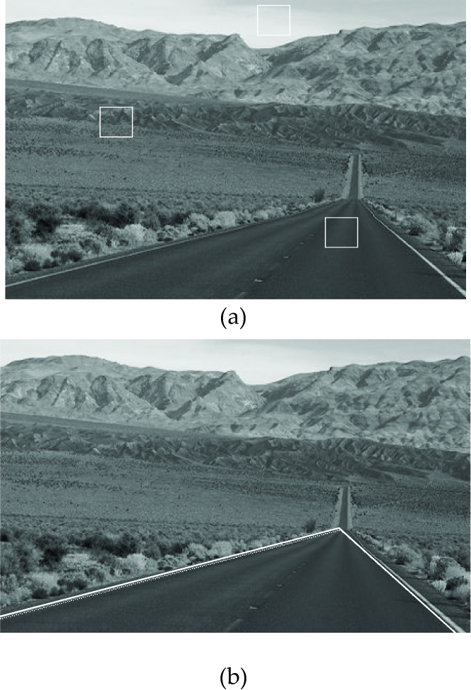
While the reflections from wet concrete shown in Fig. 12 can produce their own problems, the situation characterizing country roads with no concrete cover on the road can also produce problems related to poor separability between the road and local background. A typical example of this type is shown on Fig. 13. Now some parts of the road side banks can be added to the road area, while actually, there are no big qualitative differences between them.

Figure 13.

The example of a country road scene. Extracted borders are intensified in white.

Relevant points used for the line fitting are specified in Section 3.6 as the “leftmost on each stair on the strictly ascending part” and the “rightmost on each stair on the strictly descending part”. They are illustrated in Fig. 13.a by superimposed white circles.

Finally, we shall discuss here the abilities of the algorithm to extract the road region in a typical urban environment as is shown in Fig 14. A number of particular problems (shadows produced by trees, typical signs marking the road tracks, poor separability of the furthest part of a road etc.) are present here. While both one-dimensional approaches in classification can give acceptable results (Figures 14.a and 14.b), their combination used in two-dimensional classification shows visible improvement (Fig. 14.c), resulting in final border fitting (Fig. 14.d).

Figure 14.

The example of an urban environment: a) result obtained using statistical descriptors only; b) result obtained by structural descriptors only; c) result obtained via 2D classification; d) final result obtained after border fitting. Extracted borders are intensified in white.

6. Conclusion

The concept of an algorithm of road boundaries extraction in the context of automatic ground vehicle guidance and/or driver safety assistance systems is presented in this paper. The texture of the road region and other image regions is analysed as a source of information. Two types of descriptors, derived from the texture statistical and structural properties, are calculated and the choice of the best candidates from both categories is made in an automatic manner. The threshold values discriminating the classes are obtained by an automatic procedure of acquiring the statistical information regarding chosen descriptors.

The algorithm is generally oriented toward real-time application. This is the main reason why the number of classes is limited to three (road, near and far background), the refining by window splitting is done only around the rudimentary extracted border, the splitting is restricted down to the 16×16 window size and morphological processing steps are based on simple connectivity criteria. Two-dimensional classification was chosen in order to balance statistical and structural texture features and this approach has resulted in better extraction in comparison to a one-dimensional one. Some typical problems related to the irrelevance of third class and to the non-uniqueness of the road region texture have been analysed. In spite of the fact that there are a number of factors affecting the performances of the algorithm, it was shown that by the careful selection of algorithm steps and particular parameters it was possible to obtain promising results. Conclusions derived from these examples have led toward possible initial choices such as: 1) the region of interest is only the lower half of an image, 2) the number of classes is just two (road and non-road), 3) it is possible to obtain more than one road region and 4) it is enough to extract just one of two borders (if the other one is, for example, too short).

While the question related to the number of relevant classes is practically answered (the introduction of new classes representing more than one road region and/or more than one background region would lead toward more complex calculations, without general guarantees that the results are going to be improved), the number of descriptors can be still a subject of research. It seems that the adding of colour as the third independent feature can provide a more flexible approach in segmentation, based on chromatic contrast between road and off-road (or obstacles).

The problems discussed in this paper and the results shown are only related to the processing of static images that can be considered as an initial procedure. Basically, the algorithm should be functional in a dynamic scenario, which is the main objective of our actual and further work in this area. Dynamic nature (processing of the sequence of images) is creating some new problems, but it is also introducing some beneficial features. The variable existence of obstacles all over the road region and especially over the road border do introduce new problems. On the other hand, the extracted border, in combination with rather robust scanning/splitting procedure around it and supported by proper prediction based on results obtained in previous frames, makes the main segmentation strategy promise acceptable results again.

References

Wang

F. Y.

(Eds.) 2007, Intelligent Vehicle Vision Systems, Advanced Motion Control and Sensing for Intelligent Vehicles. Springer, 323–399

Bertozzi

Broggi

Fascioli

2000, Vision-based intelligent vehicles: State of the art and perspectives, Robotics and Autonomous Systems 32, 1–16

DeSouza

G. N.

Kak

A. C.

2002, Vision for mobile robot navigation: A survey, IEEE Transactions on Pattern Analysis and Machine Intelligence 24(2), 237–267

Gonzalez

R. C.

Woods

R. E.

2008, Digital Image Processing, Third Edition, Pearson Education, Inc.

Davies

E. R.

, Machine Vision 2005, Theory, Algorithms, Practicalities, Third Edition, Elsevier.

Bow

S. T.

2002, Pattern Recognition and Image Preprocessing, Marcel Dekker, Inc.

Lieb

Lookingbill

Thrun

Hall

2005, Adaptive Road Following using Self-Supervised Learning and Reverse Optical Flow, Proceedings of Conference-Robotics: Science and Systems, Massachusetts Institute of Technology Cambridge, Massachusetts.

Kuan

Phipps

Hsueh

A. C.

1988, Autonomous Robotic Vehicle Road Following, IEEE Transactions on Pattern Analysis and Machine Intelligence 10(5), 648–658.

Chen

K. H.

Tsai

W. H.

1997, Vision-Based Autonomous Land Vehicle Guidance in Outdoor Road Environments Using Combined Line and Road Following Techniques, Journal of Robotic Systems 14(10), 711–728

10.

Zhang

Nagel

H.-H.

1994, Texture Based Segmentation of Road Images, Proc. Symposium of Intelligent Vehicles, 260–265

11.

Rasmussen

2002, Combining Laser Range, Colour, and Texture Cues for Autonomous Road Following, Proc. IEEE Inter. Conf. on Robotics & Automation

12.

Rasmussen

2004, Grouping Dominant Orientations for Ill-Structured Road Following, Proceedings of the 2004 IEEE Computer Society Conference on Computer Vision and Pattern Recognition

13.

Oussalah

Zaatri

Van Brussel

2002, Kalman Filter Approach for Lane Extraction and Following, Journal of Intelligent and Robotic Systems 34, 195–218

14.

Wanga

Teoha

E. K.

Shen

2004, Lane detection and tracking using B-Snake, Image and Vision Computing 22, 269–280.

15.

Yang

Wang

Zhang

2002, Vision-Based Real-Time Road Detection in Urban Traffic, Proc. SPIE 4666, 75–82,

16.

Xia

T. K.

Yang

R.Q.

2006, Vision Based Global Localization for Intelligent Vehicles, Proc. of Intelligent Vehicles Symposium, 571–576

17.

Jiaa

Balasuriyaa

Challab

2008, Sensor Fusion-Based Visual Target Tracking for Autonomous Vehicles with the out-of-Sequence Measurements Solution, Robotics and Autonomous Systems 56, 157–176.

18.

Broggi

Berte

1995, Vision-Based Road Detection in Automotive Systems: A Real-Time Expectation-Driven Approach, Journal of Artificial Intelligence Research 3, 325–348.

19.

Marzotto

Zoratti

Bagni

Colombari

Murino

2010, A Real-Time Versatile Roadway Path Extraction and Tracking on an FPGA Platform, Computer Vision and Image Understanding 114, 1164–1179.

20.

Puig

Garcia

M. A.

2006, Automatic Texture Feature Selection for Image Pixel Classification, Pattern Recognition 39, 1996–2009.

21.

Garcia

M. A.

Puig

2007, Supervised Texture Classification by Integration of Multiple Texture Methods and Evaluation Windows, Image and Vision Computing 25, 1091–1106.

22.

Puig

Garcia

M. A.

Melendez

2010, Application-Independent Feature Selection for Texture Classification, Pattern Recognition 43, 3282–3297.

23.

Puig

Garcia

M. A.

Melendez

2010, Multi-Level Pixel-Based Texture Classification through Efficient Prototype Selection via Normalized Cut, Pattern Recognition 43, 4113–4123.

24.

Palm

2004, Colour Texture Classification by Integrative Co-Occurrence Matrices, Pattern Recognition 37, 965–976.

25.

Chen

Luo

Heng

P. A.

Xia

2007, Fast and Active Texture Segmentation Based on Orientation and Local Variance, Journal of Visual Communication & Image Representation 18, 119–129.

26.

Ekinci

Gibs

F. W. J.

Thomas

B. T.

2000, Knowledge-based Navigation for Autonomous Road Vehicles, Turkish Journal of Electrical Engineering 8(1)

27.

Tang

Breckon

T. P.

2011, Automatic Road Environment Classification, IEEE Transactions On Intelligent Transportation Systems 12(2), 476–484

28.

Detection of Road Image Borders Based on Texture Classification

Abstract

Keywords

1. Introduction

2. Texture Descriptors

3. Segmentation Algorithm

The Choice of the Best Candidate among Descriptors

Acquisition of Relevant Data

Definition of a Threshold

Extension to Two Dimensions

Merging/Splitting procedure

Morphological Filtration

Border Fitting

4. Verification of the Algorithm

5. Algorithm Performances and Limits

6. Conclusion

References