Sage Journals: Discover world-class research

Abstract

Nonlinear object tracking from noisy measurements is a basic skill and a challenging task of mobile robotics, especially under dynamic environments. The particle filter is a useful tool for nonlinear object tracking with non-Gaussian noise. Nonlinear object tracking needs the real-time processing capability of the particle filter. While the number in a traditional particle filter is fixed, that can lead to a lot of unnecessary computation. To address this issue, a confidence-level-based new adaptive particle filter (NAPF) algorithm is proposed in this paper. In this algorithm the idea of confidence interval is utilized. The least number of particles for the next time instant is estimated according to the confidence level and the variance of the estimated state. Accordingly, an improved systematic re-sampling algorithm is utilized for the new improved particle filter. NAPF can effectively reduce the computation while ensuring the accuracy of nonlinear object tracking. The simulation results and the ball tracking results of the robot verify the effectiveness of the algorithm.

Keywords

nonlinear object tracking adaptive particle filter confidence interval improved systematic re-sampling

1. Introduction

Nonlinear object tracking is a basic skill of mobile robotics [1]. It can improve the performance of the robot in such tasks as person following, obstacle avoidance, map building and robot localization [2 –5]. Object tracking is also a challenging task due to the presence of noise, occlusion, clutter, dynamic background elements and so on [6, 7]. The statistical method can represent ambiguity and noise in a mathematical way, and it can also give a successive object tracking result which is important for mobile robot motion control [8]. So the statistical method has become the most important object tracking method.

The Bayesian filter is a class of statistical filter technique via Bayesian inference which can recursively calculate the posterior probability, the estimated state and the predicted state [9]. The Bayesian filter is easy to implement and has a wide range of applications, so it has been extensively studied in recent years. There are several commonly used Bayesian filter methods which are applied in object tracking.

In [10], the applicability of the Kalman filter (KF) to object tracking is analysed, meanwhile the drawback of KF is also pointed in that it can only process linear system object tracking with Gaussian noise. In [11], an extended Kalman filter (EKF) is combined with a Hough transform to realize object tracking. In [12], an unscented Kalman filter (UKF) is utilized to exploit object dynamics in nonlinear systems for robust contour tracking. Both EKF and UKF are designed for nonlinear systems with Gaussian noise and their accuracy is not good enough [13]. Most object tracking problems are nonlinear systems with non-Gaussian noise, so the most useful Bayesian filter is the particle filter (PF) which can approximate random models [14].

The particle filter can handle the state estimation problem of nonlinear systems with non-Gaussian noise. The key idea of the particle filter is to use samples, also called particles, to represent the posterior distribution of the state given a sequence of sensor measurements. As new information arrives, these particles are constantly re-allocated to update the estimation of the state of the system.

While the number of particles in the traditional particle filter is fixed, that can lead to a lot of unnecessary computation and influence the efficiency of the filter [15]. So it is necessary to dynamically vary the number of particles during filtering. Some existing techniques for changing the number of particles have been presented in recent years.

In [16], a method of setting a suitable particle number according to an analysis that is carried out beforehand was proposed. This procedure considers a time-invariant particle number and assesses the quality of particle filter estimations for various sample sizes according to a Cramer-Rao bound – no sample size adaptation is conducted during the estimation process while a suitable sample size is specified in advance. The likelihood-based adaptation determines the number of samples based on the likelihood of observations during the estimation process [17]. This method is easy to implement, but it may generate particles with importance weights that are too large, which would lead to inaccurate estimation. In [18], the Kullback-Leibler distance (KLD) method is proposed to generate a more reasonable particle number adjustment. This method uses KLD to measure the distance between the true posterior density function and the empirical posterior density function, and then adapts the sample size according to the KLD. The KLD method assumes that the particles come from the true distribution while actually the particles come from an importance function. It will produce an unsuitable number of particles which would influence the accuracy of the filter. Meanwhile for hardware implementation, the KLD method is computationally too intensive. In [19], the asymptotic normal approximation method was presented. This method assumes that at each time instant of the estimation the mean and the variance satisfy an asymptotic normal approximation according to which the number of particles is produced. This method is easy to implement while it generates so few particles that the accuracy of the particle cannot be assured. In [20], the fixed empirical density quality-based method was presented. This method focuses on keeping a fixed quality of the filtering probability density function estimation. The quality of the estimation is measured by the inaccuracy between the estimation and the true probability density function, while this method is too complex to ensure the real-time process capability.

In this paper, a new adaptive particle filter algorithm is proposed which is easy to implement and can ensure certain accuracy. In this algorithm the least number of particles for the next time instant is estimated according to the confidence level and the variance of estimated state. Sampling-importance re-sampling is an essential process of particle filter which can resolve the inherent sample degeneracy problem to a certain extent. The basic idea of re-sampling is to eliminate the particles with small weights and to concentrate on the particles with large weights [21]. In this paper, an improved systematic re-sampling method is used. The algorithm we propose can effectively reduce the computation while ensuring certain accuracy.

The rest of the paper is organized as follows: Section 2 formulates the problems for object tracking. The basic idea of particle filter algorithm is presented in Section 3. Section 4 gives an adaptive adjustment of particle numbers based on confidence level. An improved systematic re-sampling method is described in Section 5. The flow of the confidence level-based new adaptive particle for nonlinear object tracking is described in Section 6. The experiment results are shown in Section 7. Section 8 generalizes the conclusion and outlines the future work.

2. Nonlinear Object Tracking Model

The generic purpose of object tracking is to track the state of a specified object or region of interest. In order to realize object tracking, two models need to be built up.

2.1 Object Motion Model

The state of an object is usually determined by the state of a previous time; therefore, the motion model of the object can be represented by a first-order discrete Markov model.

x_{t} = f (x_{t - 1}, w_{t})

(1)

where xt ∈ ℝ ^n_x denotes the states (hidden variables or parameters) of the object at time instant t; w_t ∈ ℝ ⁿ _w denotes the process noise at t; the function f: ℝ ⁿ _x * ℝ ⁿ _w ↦ ℝ ⁿ _x represent the motion models of the object; this is usually a nonlinear stochastic system.

2.2 Object Observation Model

The true state of the object cannot be obtained directly. The only thing we can obtain directly is the observation. So an observation model needs to be established in order to reveal the relationship between the observation and the states of the object.

z_{t} = h (x_{t}, v_{t})

(2)

where zt ∈ ℝ ⁿ _z denotes the observations of the object at t; v_t ∈ ℝ ⁿ _z denotes the measurement noise at t which is usually non-Gaussian; the function h: ℝ ⁿ _x * ℝ ⁿ _v ↦ ℝ ⁿ _z represents the observation model which is nonlinear.

3. Particle Filter Framework for Nonlinear Object Tracking

The particle filter is a kind of Bayesian filter algorithm which is based on the Monte Carlo simulation. This filter can effectively provide an exact, equivalent representation of the object state.

3.1 Basic Concept of the Particle Filter Algorithm

The goal of the particle filter is to estimate a posterior probability density over the state space conditioned on the data collected so far. It is a variant of the Bayesian filter which uses a set of particles S_t with associated weight to represent or approximate the posterior distribution.

S_{t} = {〈 x_{t}^{i}, w_{t}^{i} 〉 | i = 1, …, n}

(3)

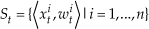
where t means the time instant; x_tⁱ is the i^th particle's state and w_tⁱ is a non-negative numerical factor called the importance weights of the i^th particle at t, these weights sum up to one; n is the total number of the particles. These particles are sampled from the posterior density. There is a relationship between the posterior density and the particle importance weight. If a particle is sampled from the high density region, the importance weight of the particle is big.

3.2 Particle Filter-Based Nonlinear Object Tracking

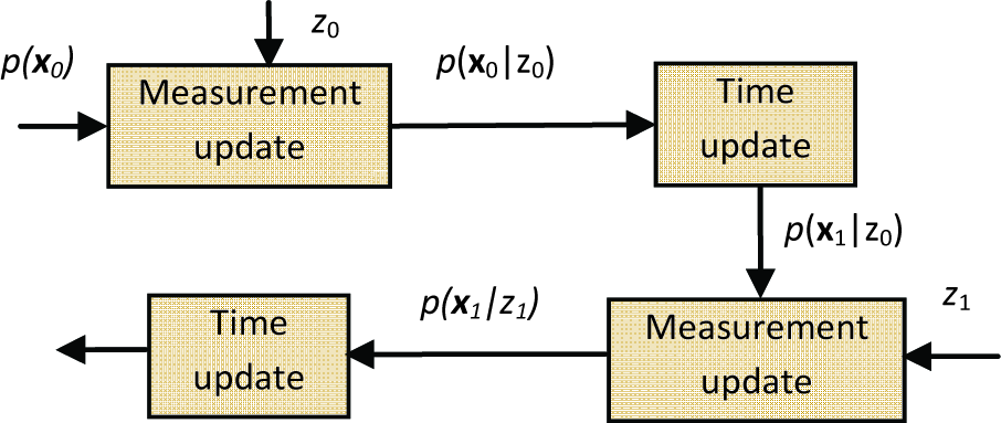
The nonlinear object tracking problem is difficult because the true state of the object is hidden by noisy observations. The particle filter is adapted to nonlinear state estimation with Gaussian or non-Gaussian noise. So particle filter is suitable for nonlinear object tracking. The aim of object tracking is to evaluate the posterior probability function p(x_t | z_t) and then obtain an estimation of x_t. Usually this process can be accomplished by two steps iteratively, the time update step and the measurement update step, as shown in Figure 1. When the new measurement and the result of time update step in the last time instant are obtained, the measurement update step works, then the result of this step will be utilized in the next update step.

Figure 1.

Update step of PF-based nonlinear object tracking

(1) Time update

Obtain the state transition probability p(x_t–₁ | z_t–₁) according to (1). p(x_t–₁ | z_t–₁) is already known and then p(x_t | z_t–₁) can be calculated using (4).

p (x_{t} | z_{t - 1}) = \int p (x_{t} | x_{t - 1}) p (x_{t - 1} | z_{t - 1}) d x_{t - 1}

(4)

(2) Measurement update

In this step the observation model information p(z_t | x_t) at time t is used to update p(x_t | z_t–₁) according to Bayesian inference (5).

p (x_{t} | z_{t}) = \frac{p (z_{t} | x_{t}) p (x_{t} | z_{t - 1})}{\int p (z_{t} | x_{t}) p (x_{t} | z_{t - 1}) d x_{t}}

(5)

In the particle filter Equation (5) can be approximated with (6).

p (x_{t} | z_{t}) \propto p (z_{t} | x_{t}) p (x_{t} | z_{t - 1}) \approx \sum_{1}^{N} ω_{t}^{i} δ (x_{t} - x_{t}^{i})

(6)

δ(.) is a Dirac Delta function and ωⁱ_t can be recursively updated with (7).

ω_{t}^{i} \propto ω_{t - 1}^{i} p (z_{t} | x_{t}^{i})

(7)

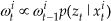
Then normalize ωⁱ_t using (8)

ω_{t}^{i}^{*} = \frac{ω_{t}^{i}}{\sum_{1}^{N} ω_{t}^{i}}

(8)

3.3 Flow of Particle Filter-Based Nonlinear Object Tracking

The flow of particle filter-based nonlinear object tracking is shown as below:

(1) t=0 i=1 do Initialization: draw the states x₀ⁱ from the prior p(x₀) //x₀ is the initial state of the object while (i++<=n) (2) for t = 1,…,tf: // tf is the run time of the NAPF i=1 do Generate particle xⁱ_t from q(x_t | xⁱ_0:t–1, y_1: _t) while (i++<=n) i=1 do Evaluate the importance weights according to ( 7 ) while (i++<=n) i=1 do Normalize the importance weights according to ( 8 ) while (i++<=n) i=1 do Resampling: multiply/suppress samples xⁱ_t with high/low importance weights ωⁱ_t respectively, to obtain n random particles x˜ⁱ_t while (i++<=n) i=1 do Set

{\tilde{w}}_{t}^{i} = \frac{1}{n}

, where w˜ⁱ_t is the weight of x˜ⁱ_t while (i++<=n)

Output: output the estimate of x_t which can be obtained straight forwardly by (9).

x_{t}^{} = \sum_{i = 1}^{n} {\tilde{x}}_{t}^{i} {\tilde{w}}_{t}^{i} = \frac{1}{n} \sum_{i = 1}^{n} {\tilde{x}}_{t}^{i}

(9)

4. Adaptive Adjustment of Particle Number Based on Confidence Level

Nonlinear object tracking is an essential task of robotics which requires on-line processing of a large amount of data, so it is necessary to reduce computation time and improve real-time performance.

In traditional particle filter algorithms, the number of particles is fixed which can decide the computation time. It is possible that fewer particles can meet the required performance. In this paper we propose an adaptive adjustment method based on the confidence level.

In the theory of probability, the concept of the confidence interval reveals the relationship between the number of samples and the estimation accuracy [22]. The confidence interval can contain the estimated parameter with the probability confidence level.

For the variance of particle filter, the central limit theorem justifies an asymptotic normal approximation for it. This is given by (10):

E_{P F} (x) \sim N (E_{p} (x), σ_{P F}^{2} / M_{P F})

(10)

where N(μ,σ²) denotes the normal distribution with mean ì and standard derivation σ. E_p(x) is the true mean value of the estimated state. E_PF(x) is the estimated state by particle filter. σ_PF² is the variance of the particle state. M_PF is the particle number which can be adaptively adjusted.

Assume that the confidence level is 1 – α, according to the concept of confidence interval, Equation (11) can be obtained:

\begin{array}{l} P (E_{p} (x) - z_{α / 2} (\frac{σ}{\sqrt{N_{P F}}}) < E_{P F} (x) < E_{p} (x) + \\ + z_{α / 2} (\frac{σ}{\sqrt{N_{P F}}})) = (1 - α) \end{array}

(11)

Er is the maximum error of the estimation that satisfies the confidence level 1 – α.

E r = z_{α / 2} (\frac{σ}{\sqrt{M_{P F}}})

(12)

Given the error of particle filter estimation å, set Er is equal to å, then

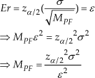
\begin{array}{l} E r = z_{α / 2} (\frac{σ}{\sqrt{M_{P F}}}) = ε \\ \Rightarrow M_{P F} ε^{2} = z_{α / 2}^{2} σ^{2} \\ \Rightarrow M_{P F} = \frac{z_{α / 2}^{2} σ^{2}}{ε^{2}} \end{array}

(13)

So under the qualification of confidence level1 – α, the number of efficient particles is $\frac{z_{α / 2}^{2} σ^{2}}{ε^{2}}$ .

5. Improved Systematic Re-sampling Used for the New Adaptive Particle Filter

5.1 Sequential Importance Re-sampling

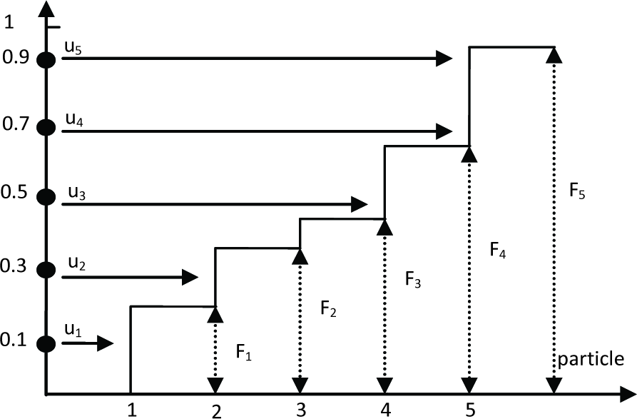
Sequential importance re-sampling is an essential process of the particle filter which can resolve the inherent sample degeneracy problem to some degree. The basic idea of re-sampling is to eliminate the particles with small weights and to concentrate on the particles with large weights.

Figure 2 shows the re-sampling process of the particle filter. The size of the dot represents the importance weight. At the beginning the original particles have the same weights which are generated from the previous time re-sampling. Using Equation (8) the weights are updated which reflect the importance of the particles according to the posterior density. In the re-sampling step, the particles with big weights will be multiplied several times, while the particles with small weights will be eliminated. Ascertaining how to select the multiplied particles is therefore essential.

Figure 2.

Re-sampling of particle filter algorithm

Currently there are four important re-sampling methods for the particle filter: multinomial re-sampling, stratified re-sampling, systematic re-sampling and residual re-sampling [23–24].

Multinomial re-sampling is the simplest and earliest re-sampling method, it divides the re-sampling space into n random sub-spaces, where n is the number of particles. Stratified re-sampling divides the re-sampling space into n disjoint sub-spaces of the same size and each sub-space will generate a re-sampled particle with a random position in the sub-space. The only difference between systematic re-sampling and stratified re-sampling is that the particles re-sampled by the systematic re-sampling method have the same position in each sub-space. In residual re-sampling, the resample space concept and random number are not utilized which makes it different from the above methods. Residual sampling is a mostly deterministic approach that enforces the number of copies of a particle according to the weight of the particle.

5.2 Improved Systematic Re-sampling

Among the four re-sampling methods, the performance of systematic re-sampling is the best because it has the least computation complexity. Thus, systematic re-sampling is proposed as a basic particle filter whose particle number is fixed during filtering. So systematic re-sampling has to be properly modified to be applied in NAPF whose particle number may change in each time instant.

Systematic re-sampling stratifies the sampling space into n subspaces where each sample has the same position. In a traditional particle filter n is a constant, while in NAPF the number of particles is a variable which is adaptively adjusted according to Equation (13).

Assume that M^t_PF is the particle number at time t. The process of the improved systematic re-sampling is shown as follows:

(1) Obtain an ordered random number

u_{j} = \frac{(j - 1)}{M_{P F}^{t}} + U

(14)

U is a single random number drawn from [0,1 / M^t_PF), 1 ≤ j ≤ M^t_PF.

(2) Set $F_{i} = \sum_{m = 1}^{i} w_{t}^{m}, 1 \leq i \leq M_{P F}^{t}$ , calculate X_j which is the number of u_j that lies in the interval (F_i_–1,F_i].

(3) Replicate x_t^j X_j times, X_j > 0.

(4) Obtain new particle sets S_t.

S_{t} = {〈 x_{t}^{i}, w_{t}^{i} 〉 | i = 1, …, M_{P F}^{t}}

(15)

The systematic re-sampling can be explained in Figure 3. Figure 3 is an example of systematic re-sampling with five particles and U is 0.1.

Figure 3.

Systematic re-sampling for an example with five particles

6. Flow of Confidence Level-Based New Adaptive Particle Filter for Nonlinear Object Tracking

In order to avoid frequently re-sampling and reduce unnecessary computation, a threshold R is introduced. Meanwhile N_min is a bound of the particle number, if the number of particles generated by NAPF is smaller than N_min, the number of particle for the next time instant will be set to be N_min; N_max is the original number of particle number which is also the maximum number during the NAPF. This method can assure the accuracy of the particle filter. The flow of the confidence level-based new adaptive particle for nonlinear object tracking is as follows:

(1) t = 0 i =1 do Initialization: draw the states xⁱ₀ from the prior p(x₀) while (i++ <= n) (2) for t = 1,…, tf. // tf is the run time of the NAPF i=1 do Genetate particle x_tⁱ from q(x_t | xⁱ_0:t–1, y_1:t) while (i++<=M^t_PF) i =1 do Evaluate the importance weights according to ( 7 ) while (i++<=N^t_PF)

Output: output the estimate of the x_t which can obtained straight forwardly by (16)

x_{t}^{} = \sum_{i = 1}^{n} {\tilde{x}}_{t}^{i} {\tilde{w}}_{t}^{i} = \frac{1}{n} \sum_{i = 1}^{n} {\tilde{x}}_{t}^{i}

(16)

Particle number adjustment: obtain the number of particles N_PF^t+1 according to (13), then choose the proper number of N_PF^t+1

if M_PF^t+1 ⩾ N_max M_PF^t+1 = N_max else if M_PF^t+1 ⩽ N_min M_PF^t+1 = N_min else M_PF^t+1 = M_PF^t+1

Improved systematic re-sampling step:

if |M_PF^t+1 – M_PF^t|⩽R No re-sampling else Improved systematic re-sampling i=1 do Normalize the importance weights according to ( 8 ) while (i++<=M^t_PF)

7. Experiment Results

7.1 Simulation Results

In the simulation, we assume that the motion model and the observation model of the object tracking are nonlinear systems which are shown as follows:

\begin{array}{l} x_{k} = 0.5 x_{k - 1} + 25 x_{k - 1} / (1 + x_{k - 1}^{2}) + 8 \cos (1.2 * (k - 1)) + w_{t} \\ y_{k} = x_{k}^{2} / 20 + v_{t} \end{array}

Assume that w_t and v_t are white Gaussian noise with variance 10 and 1. The initial number of particles is set to be 500 which is also the maximum number of particles during the estimation. We compare the NAPF with EKF, UKF and the traditional PF. The confidence level is 95%; given the error of particle filter estimation ε is equal to 16. The time step is 50 because it can give a relatively clear state estimation figure.

Estimation error (ER) is obtained from Equation (17)

E R = | x - \bar{x} |

(17)

where x is the true state of the object, x̄ is the estimated state of the object. ER can reflect the estimation accuracy. From Figure 4 and Figure 5 we can see that the estimation of EKF is not satisfying. EKF only uses the first order terms of the Taylor series expansions of the nonlinear functions. So it often introduces large errors in the estimated statistics of the posterior distributions of the states if the system is strongly nonlinear. UKF does not approximate the nonlinear process and observation models; it uses the true nonlinear models and approximates the distribution of the state random variables using the scaled unscented transformation. UKF's performance is better than EKF, while the estimation of UKF is only accurate to the second order of the Taylor series expansion. The particle filter uses a set of particles to represent the posterior distribution. From Figure 4 we find that it obtains the best performance, while NAPF also acquires relatively good accuracy.

Figure 4.

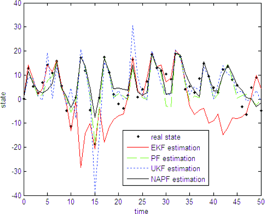
Object estimation results of EKF, UKF, PF and NAPF in 50 time steps

Figure 5.

ER of EKF, PF, UKF and NAPF for 50 random realizations

In Figure 6 we can see that NAPF estimation almost lies in the 95% confidence interval. That is because NAPF adjusts the number of particle filter adaptively according to the estimation quality which can ensure a certain accuracy of object tracking.

Figure 6.

NAPF estimation and 95% confidence interval

The root mean square error (RMSE) is another value that can be used to reflect the accuracy of object state estimation.

R M S E_{} = \sqrt{\frac{\sum_{t = 1}^{t_{f}} {(x - \bar{x})}^{2}}{t_{f}}}

(18)

We have run EKF, UKF, PF and NAPF for 10000 time steps, the RMSE of the four algorithms are shown in Table 1. From Table 1 we can obtain a similar conclusion to that from Figure 4 and Figure 5.

Table 1.

RMSE of four algorithms

ALGORITHM	EKF	UKF	PF	NAPF
RMSE	15.7732	6.6243	4.9637	5.7825

In order to reveal the runtime reduction of NAPF, we run PF and NAPF for 10000 time steps, then obtain the average run time and particle number of each step, the results are shown in Table 2. NAPF can reduce the particle number by about 24.7%, while the runtime of the particle number is reduced by about 23.6% – that is because the improved re-sampling of NAPF will consume some runtime.

Table 2.

Elapsed time of 50 time steps

Algorithm	PF	NAPF
Particle number	500	376.6
Average time	1.665ms	1.271ms

7.2 Object Tracking Results

We hereafter experimentally validate the effectiveness of NAPF for a real robot's object tracking. The robot “Education robot” developed by Chinese Academy of Sciences is utilized to realize ball tracking, as shown in Figure 7. The tracking of the ball is realized by a camera. We assume that the robot can obtain accurate self-localization. The picture is obtained by an ultra-high definition colour gun camera AMPSON DSC-B468C and is processed using an FPGA Cyclone II EP2C20. The image pixel of the picture obtained by the camera is 256*256. In one second about 30 pictures can be processed.

Figure 7.

NAPF estimation and 95% confidence interval

In each time instant, the ball is assumed to move in a uniform rectilinear motion, the motion model and observation model are shown as below:

\begin{array}{l} x_{k} = x_{k - 1} + \frac{(x_{k - 1} - x_{k - 2})}{Δ t} \times Δ t + w_{t} = x_{k - 1} + (x_{k - 1} - x_{k - 2}) + w_{t} \\ y_{k} = x_{k} + v_{t} \end{array}

Assume that w_t is the process noise and v_t is the measurement noise. Both of them are random noise.

Δt is the time instant and our experiment is 30ms.

The ball tracking experiment was implemented in an empty room which is about 5m*4.9m. The ball tracking results are shown in Figure 8. From Figure 8 we can find that both PF and NAPF can give ideal ball tracking results, while the estimation of PF is more exact than NAPF. In our experiment of each frame image the mean runtime of PF is 2.61 ms, the mean runtime of NAPF is 1.98 ms. So we can conclude that NAPF can effectively reduce the runtime while ensuring certain accuracy of nonlinear object tracking.

Figure 8.

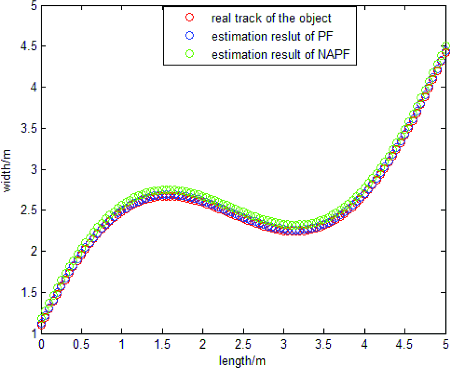
The ball tracking result of PF and NAPF

8. Conclusions and Future Work

In this paper, we have presented a new adaptive particle filter algorithm for nonlinear object tracking. During each time instant of the particle filter, the idea of confidence interval is utilized to estimate the least number for the next time instant. This can reduce unnecessary computation of the particle filter and then enhance the adaptation which is essential for real-time nonlinear object tracking. Accordingly, a systematic re-sampling method is modified to accommodate the adaptive particle filter. The experiments indicate that NAPF can effectively reduce the computation while ensuring certain accuracy. In future work, we will research how to further reduce the computation and runtime of the particle filter and how to increase the accuracy.

Footnotes

9. Acknowledgements

This paper is supported by the National Natural Science Foundation of China (nos. 61071096 and 61073103), Research Fund for the Doctoral Programme of Higher Education of China (nos. 20110162110042 and 20100162110012), the Science and Technology Planning Project of Hunan Province, China (no. 2011GK3214).

References

Yilmaz

Javed

Shah

(2006) Object Tracking: A Survey. ACM Computing Surveys. 38, 4, 1–45

Chen

Birchfield

(2007) Person Following with a Mobile Robot Using Binocular Feature-Based Tracking. Proceedings of the 2007 IEEE International Conference on Intelligent Robots and Systems, 815–820, October, 2007, IEEE International Conference on Intelligent Robots and Systems, San Diego, California, USA

Chunyu

Pollak

Falash

(2009) A New Reactive Target-tracking Control with Obstacle Avoidance in a Dynamic Environment. Proceedings of the 2009 American Control Conference, 3872–3877, American Control Conference 2009, Orlando, Florida, USA

Bacca

Salvi

Cufi

(2010) Mapping and Localization for Mobile Robots through Environment Appearance Update. Proceedings of the 2010 Conference on Artificial Intelligence and Development, 291–300, Conference on Artificial Intelligence and Development, Espluga de Francoli, Spain

Corke

Detweiler

Dunbabin

Hamilton

Rus

Vasilescu

(2007) Experiments with Underwater Robot Localization and Tracking. Proceedings of the 2007 IEEE International Conference on Robotics and Automation, 4556–4561, April, 2007, IEEE International Conference on Robotics and Automation 2007, Roma, Italy

Koohi

Narghi

Shakey

(2011) An Algorithm for Object Tracking Based on Adaptive Triangle Shape Mesh Estimation Method. Canadian Journal on Image Processing and Computer Vision. 2, 1, 354–359

Papadourakis

Argyros

(2010) Multiple Objects Tracking in the Presence of Long-term Occlusions. Computer Vision and Image Understanding. 114, 7, 835–846

Erickson

Knuth

Okane

Lavalle

(2008) Probabilistic Localization with A Blind Robot. Proceedings of IEEE International Conference on Robotics and Automation, 1821–1827, May, 2008. IEEE International Conference on Robotics and Automation, California, USA

Zivkovic

Cemgil

Krose

(2009) Approximate Bayesian Methods for Kernel-based Object Tracking. Computer Vision and Image Understanding. 113, 6, 743–749

10.

Funk

(2003) A Study of the Kalman Filter Applied to Visual Tracking. Technical Report. University of Alberta

11.

Mills

Pridmore

Hills

(2004) Tracking in a Hough Space with the Extended Kalman Filter. Proceedings of the 2003 International Conference on Pattern Recognition, 173–182, August, 2004, International Conference on Pattern Recognition, Cambridge, UK

12.

Chen

Rui

Huang

(2006) Multicue HMM-EKF for Real-time Contour Tracking. IEEE Transaction on Pattern Analysis and Machine Intelligence. 28, 9, 1525–1529

13.

Giannitrapani

Ceccarelli

Scortecci

Garulli

(2011) Comparison of EKF and UKF for Spacecraft Localization via Angle Measurements. IEEE Transactions on Aerospace and Electronic Systems, 47, 1, 75–84

14.

Hendeby

Karlsson

Gustafsson

(2010) Particle Filtering: The Need for Speed. EURASIP Journal on Advances in Signal Processing, 2010, 22, 1–9

15.

Doucet

Arnaudismacjp

Johansen

(2009) A Tutorial on Particle Filtering and Smoothing: Fifteen Years Later. Handbook of Nonlinear Filtering. 1, 12, 4–6

16.

Simandl

Straka

(2002) Nonlinear Estimation by Particle Filters and Cramer-rao Bound. Proceedings of the 15th Teiennial World Congress of International Federation of Automatic Control, 79–84, October, 2002, Teiennial World Congress of International Federation of Automatic Control, Barcelona, Spain

17.

Fox

Burgard

Dellaert

Thrun

(1999) Monte Carlo Localization: Efficient Position Estimation for Mobile Robots. Proceedings of the 1999 National Conference on Artificial Intelligence, 343–349, July, 1999, National Conference on Artificial Intelligence Orlando, Florida, USA

18.

Fox

(2003) Adapting the Sample Size in Particle Filters Through KLD-Sampling. International Journal of Robotics Research. 22, 985–1003

19.

Soto

(2005) Self Adaptive Particle Filter. Proceedings of the 2005 International Joint Conference on Artificial Intelligence, 1398–1406, August, 2005, International Joint Conference on Artificial Intelligence, Edinburgh, Scotland

20.

Straka

Simandl

(2008) Adaptive Particle Filter with Fixed Empirical Density Quality. Proceedings of the 17th Teiennial World Congress of International Federation of Automatic Control, 6484–6489, July, 2008, Teiennial World Congress of International Federation of Automatic Control, Seoul, Korea

21.

Jia

(2010) An Improvement on Resampling Algorithm of Particle Filter. IEEE Transactions on Signal Processing, 58, 10, 5414–5420

22.

Shao

(2007) Mathematical Statics (2nd Edition). Springer

23.

Sattar

Sun

(2012) Deterministic resampling: Unbiased Sampling to Avoid Sample Impoverishment in Particle Filter. Signal Processing, 92, 7, 1637–1645

24.

Douc

Cappe

(2005) Comparison of Resampling Schemes for Particle Filtering. Proceedings of 14th International Symposium on Image and Signal Processing and Analysis, 64–69, September, 2005, International Symposium on Image and Signal Processing and Analysis, Palaiseau, France

Confidence-Level-Based New Adaptive Particle Filter for Nonlinear Object Tracking

Abstract

Keywords

1. Introduction

2. Nonlinear Object Tracking Model

2.1 Object Motion Model

2.2 Object Observation Model

3. Particle Filter Framework for Nonlinear Object Tracking

3.1 Basic Concept of the Particle Filter Algorithm

3.2 Particle Filter-Based Nonlinear Object Tracking

(1) Time update

(2) Measurement update

3.3 Flow of Particle Filter-Based Nonlinear Object Tracking

4. Adaptive Adjustment of Particle Number Based on Confidence Level

5. Improved Systematic Re-sampling Used for the New Adaptive Particle Filter

5.1 Sequential Importance Re-sampling

5.2 Improved Systematic Re-sampling

6. Flow of Confidence Level-Based New Adaptive Particle Filter for Nonlinear Object Tracking

7. Experiment Results

7.1 Simulation Results

7.2 Object Tracking Results

8. Conclusions and Future Work

Footnotes

9. Acknowledgements

References