Sage Journals: Discover world-class research

Abstract

Audio-visual speech recognition is a natural and robust approach to improving human-robot interaction in noisy environments. Although multi-stream Dynamic Bayesian Network and coupled HMM are widely used for audio-visual speech recognition, they fail to learn the shared features between modalities and ignore the dependency of features among the frames within each discrete state. In this paper, we propose a Deep Dynamic Bayesian Network (DDBN) to perform unsupervised extraction of spatial-temporal multimodal features from Tibetan audio-visual speech data and build an accurate audio-visual speech recognition model under a no frame-independency assumption. The experiment results on Tibetan speech data from some real-world environments showed the proposed DDBN outperforms the state-of-art methods in word recognition accuracy.

Keywords

Audio-visual speech recognition Deep Dynamic Bayesian Network unsupervised feature learning Tibetan speech recognition

1. Introduction

The field of Human Robot Interaction (HRI) is moving from safe and functional interactions to socially assistive and natural interactions. One important application is to design and implement intelligent and automatic agents to naturally interact with users in their daily work and life, in order to improve their quality of life and health. While different modes of interaction have been developed including traditional keyboards, mice and recent development on body gesture based interactions such as the Kinect sensor, the most natural interaction mode between human and robot remains speech, in particular for elderly people and for people with disability. Speech recognition however, remains challenging, in particular in a natural setting. The problem can be exacerbated for certain minority language, such as Tibetan language, where very few benchmark datasets are available for training the algorithms and data collection and annotation is also difficult. In this paper, we intend to address this challenge by proposing a multi-modal deep learning framework for Tibetan speech recognition.

The approaches of multimodal pattern recognition may be classified into three categories: feature fusion (or early integration), decision fusion (or late integration) and model fusion (or middle integration). In the case of model fusion, various heuristic-based combination strategies are used to form a unified Dynamic Bayesian Network (DBN) model from separately trained HMMs [1]. At this time model fusion seems to be the best technique to integrate information from multi-modality.

For speech recognition, phonemes from audio data and visemes (lip shape and motions) from visual data are correlated at a “mid-level”. In recent works, a multi-stream DBN model and coupled HMM are popular methods for the middle integration [1 ]–[4]. They make use of a single audio stream HMM and a single video stream HMM and integrate the information from multiple audio and visual streams. However, as we know, in HMM models the features of the audio and visual signals are independent among the frames. However, studies [5] have shown that context-dependency among audio and visual observations exists.

In [6], the deep belief networks based on restricted Boltzmann machines were applied to deal with the inter-frame dependency of audio-visual data, by the unsupervised learning of shared features between modalities. However, deep belief networks have some inherent weaknesses. First, the number of hidden nodes in each layer is set before learning. Under no prior knowledge of phonemes and visemes, this may result in redundant or missing features. Second, there are no lateral connections among the hidden nodes. While simplifying the learning, this assumption fails to capture strong feature dependences. Third, it cannot capture the temporal relationships among random variables. However, the basic pattern for audio and visual data varies in time [7].

Tibetan is such a complex language that its linguistic study remains primitive. In fact, there is little linguistic knowledge so far on Tibetan speech recognition. In this paper we propose a Deep DBN to learn Tibetan acoustic features, visual features and their shared representation, without any prior linguistic knowledge of Tibetan phonemes and visemes, based on which we propose to build an accurate audio-visual speech recognition model, without assuming inter-frame independency among features.

Specifically, we introduce an unsupervised method to learn the spatial-temporal features for audio data, visual data and shared representation based on DDBN. The proposed method can learn the features automatically. We apply the learned features to speech classification of isolated letters, digits and words. The experimental results show that the DDBN recognition models based on the learned features have a significant improvement in performance over the commonly used multi-stream DBN and coupled HMM.

The remainder of this paper is structured as follows. In section 2 we briefly introduce the Deep Dynamic Bayesian Network and the proposed DDBN topology for audio-visual speech features learning and speech recognition. Section 3 discusses the unsupervised learning features strategy we proposed. In section 4, we first discuss our audio and video data pre-processing methods. We then analyse experimental results on Tibetan audio-visual speech classification. This paper concludes in section 5, which offers conclusions and directions for future work.

2. Deep Dynamic Bayesian Network

DBNs are hierarchical probabilistic graphical models that are often used to capture the spatial-temporal relationships among random variables at different levels of abstraction. DBNs represent a generalisation of the widely used dynamic models including HMMs, Kalman filtering and linear Dynamic Systems [8].

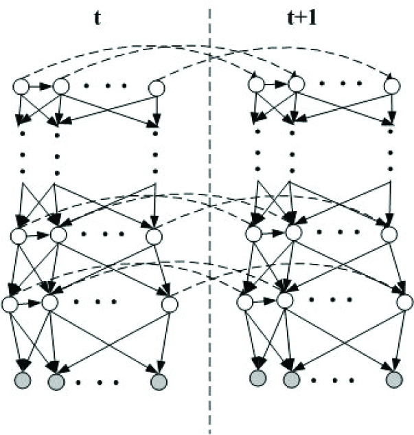
A DBN topology includes two parts; the spatial part and the transition part, as shown in Figure 1 (a) and (b). The spatial part captures the spatial relationships among different random variables, while the transition part captures the dynamic dependencies among the random variables. Learning a DBN topology requires learning both the spatial and transition parts.

Figure 1.

An example DBN with (a) a spatial network, and (b) a transition network

With DBN, a complex pattern can be broken down into atomic components at different levels and the relationships among these elements can be captured by the links among them. Therefore, we propose to develop a deep DBN framework, as shown in Figure 2, to represent complex space-time object patterns. With the framework, a complex pattern is composed of elemental components of different complexities at different levels of abstraction, with the output of the previous layer serving as the input of the current layer. The output of each layer succinctly and invariantly summarises its input through spatial and temporal links. Starting from the first layer, whose input includes the sensory data/features (e.g. audio/acoustic features, image/image features), the elemental components in each layer become progressively more complex and abstract until the final layer, which represents the complex object patterns.

Figure 2.

The topology of deep DBN

It is the elemental components in different layers and their spatial-temporal interactions with each other that jointly compose the complex object patterns we want to recognise. Such a hierarchical model gives a rich representation of the complex patterns and its ability to compose elements hierarchically can be a powerful way to manage complexity and promote scalability and extensibility.

Based on the proposed DDBN topology, we present an audio-visual speech recognition model as shown in Figure 3. In this model, the first (the bottom) layer represents the raw data as the input, including audio and visual data. The second layer is hidden and represents the features extracted from audio modality and visual modality separately. The third layer consists of the shared features learned from acoustic and visual features. All features in the second and third layers will be learned by unsupervised learning. The top layer represents the speech label node, which links with the nodes in the shared features layer. Meanwhile, considering the dynamic inter-frame dependency among features, we assume the feature variables, as well as label variable, form a first order Markov chain as illustrated in Figure 3.

Figure 3.

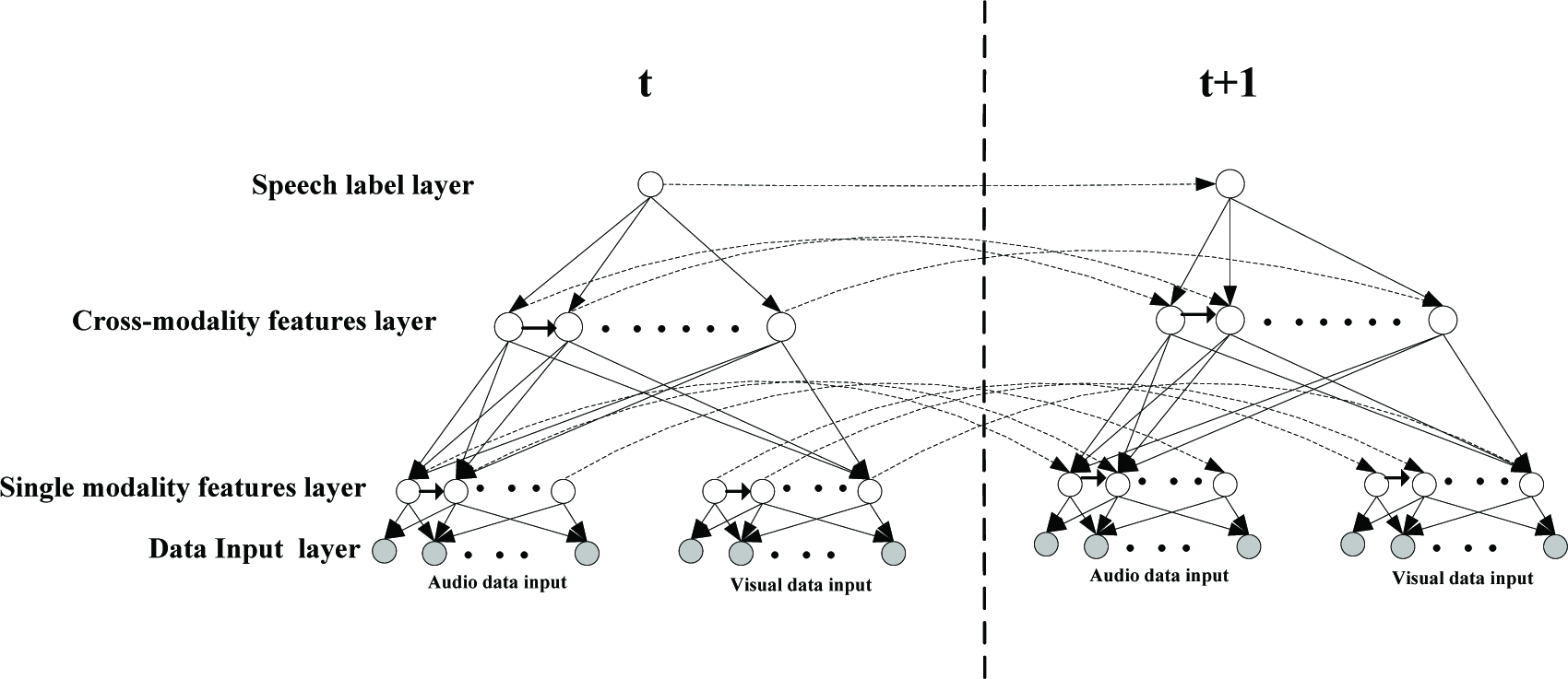
A DDBN topology for features learning and audio-visual speech recognition

Assuming that the low dimensional feature vectors are embedded in raw signal [9], we define each feature node as a hidden continuous state variable of l dimension. The output of the single modal feature layer and the shared feature layer is composed of multiple feature nodes of this type.

In Figure 3, assume x_i^t is the i th node of data input layer in time slice t, from which we would extract single modality features. The hidden variable h_k^w^,t represents the kth feature node of the wth hidden layer in time slice t. s^t denotes the discrete utterance label node in the top layer. According to the proposed DDBN's topology for audio-visual speech recognition, the probability distribution over label variable is

P (s^{t} = z) = \sum_{l = 1}^{L} P (s^{t} = z | s^{t - 1} = l) p (s^{t - 1} = l),

(1)

and the joint probability distribution over input variables ({x^t_i}) features ({h_k^w^,t}) and labels ({st}) is

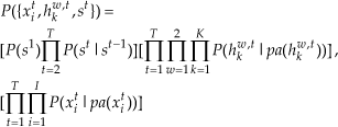
\begin{array}{l} P ({x_{i}^{t}, h_{k}^{w, t}, s^{t}}) = \\ [P (s^{1}) \prod_{t = 2}^{T} P (s^{t} | s^{t - 1})] [\prod_{t = 1}^{T} \prod_{w = 1}^{2} \prod_{k = 1}^{K} P (h_{k}^{w, t} | p a (h_{k}^{w, t}))], \\ [\prod_{t = 1}^{T} \prod_{i = 1}^{I} P (x_{i}^{t} | p a (x_{i}^{t}))] \end{array}

(2)

where pa(*) are the parents of node*.

The main strengths of the proposed DDBN framework for audio-visual speech recognition lie in its hierarchical structure, its capability of decomposing a speech recognition problem into elemental components at different levels, its capability of capturing the spatial-temporal relationships among features variables at different levels and its capability of handling the associated uncertainties and dynamics at each layer. It allows multimodal information integration at middle level. In addition, the hierarchical structure matches well with the process that a human uses for audio-visual speech pattern representation and recognition. These features are important for the proposed deep learning paradigm.

3. DDBN topology and the features learning for audio-visual speech recognition

Given our understanding of the DBN, we present the following method to learn a DDBN topology in an unsupervised manner. This method can be used for acoustic features, visual features and shared features. In this section we describe how to construct the DDBN topology for the audio-visual speech recogniser. The DDBN topology learning consists of two steps: the spatial networks and the transition networks.

3.1 Learning spatial networks

For the spatial network we need to learn the topology block by block (as shown in Figure 4), starting from the first block (the bottom layer and the next higher layer). In each block we need to learn the number of output nodes (feature nodes) and the structure between the input nodes and output nodes.

Figure 4.

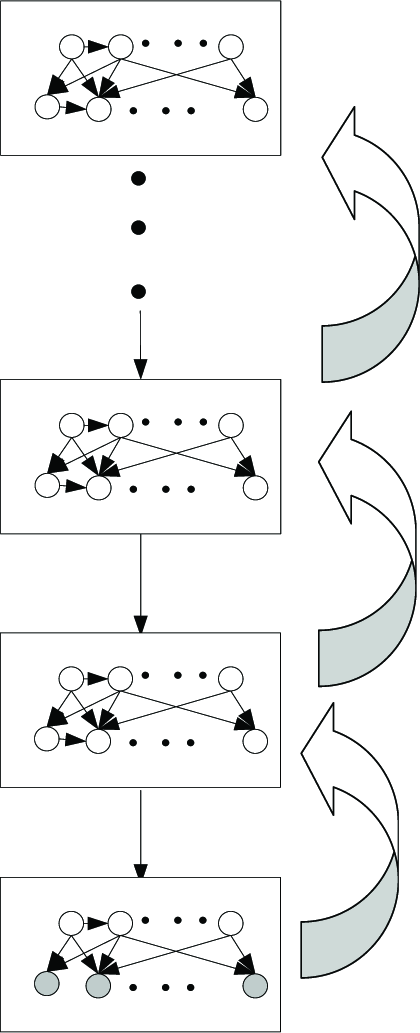
Spatial networks learning

3.1.1 Features learning

Within one block, given its input, we first determine the number of nodes in its output using a greedy approach. The approach starts with one output node. It then uses the structure learning approach (to be discussed later) to learn the optimal structure. This process then repeats, with one output node being added each time and computing the corresponding optimal structure. The process stops when the score of the estimated optimal structure does not improve anymore.

3.1.2 Structure learning

Given the number of output nodes in a block, a method is needed to learn the topology for a block. For this we will apply the structural Expectation Maximisation (EM) method [10] to determine the links between the input nodes and the output nodes for a block.

To illustrate the EM method for learning in one block, we use Figure 5, where B nodes are the input nodes and A nodes are the output nodes for the block. The input nodes (B) are given, while the output nodes (A) are hidden and unlabelled. The goal of structure learning is to learn the links among nodes A and B. We rely on a structural EM framework to learn the arcs among A and B. A typical EM method consists of two steps; E-step and M-step. The E-step computes the expected values for the hidden nodes (A), given the current structure of the network, while the M-step applies such expected statistics to learn a new structure by maximisation of its likelihood. This is done iteratively until no improvement in the structure can be achieved. A summary of the structural EM algorithm is as follows:

Figure 5.

Learning the structure (links) of one block, where (a) is the initial structure, and (b) is the desired structure

Choose an initial structure G₀ and estimate the parameters θ₀ for G₀

For t = 0, 1… until convergence

“Complete the data” - Compute the expected values of the variables with structure G_t and parameter θ_t

Find the structure G_t₊₁ that maximise the score (BIC, BDe etc.) of the two-layer network through a greedy hill climbing procedure

Learn the parameter θ_t+1 for G_t₊₁ with the parameter EM algorithm

Once a block is learned we can sample its output nodes to produce new input data for the next higher layer. This process is then repeated for the next block and continues until the final block.

3.1.3 Spatial networks learning for the audio-visual speech recognition model

For an audio-visual speech recognition model based on DDBN, we first learn two parallel blocks' topologies, between the raw data input layer and the single modality features layer, one for audio data and one for visual data. The audio block captures the relationships among the raw audio input data and extracted acoustic features nodes, while the video block captures the relationships among raw visual input data and extracted visual features. Take the audio block, for example, given the N input nodes, we must first determine the number of nodes in the feature layer using a greedy approach. The approach starts with one feature node. It then uses the structure EM learning approach to learn the structure. This process then repeats, with one feature node being added each time and the corresponding structure being computed. The process stops when the score of the estimated block structure does not improve anymore.

After the topologies of two single-modal blocks are found, the extracted acoustic features and visual features will serve as the input nodes for the next higher block, in which the cross-modality features are learned. We repeat the same block learning procedure to obtain new nodes at the shared features layer and the topology between the single modality features layer and the shared features layer.

In the top block we construct a classifier between the shared features layer and the label layer by linking the label node to all shared feature nodes. So far, we have learnt the spatial network of the proposed DDBN for audio-visual speech recognition, as shown in Figure 6.

Figure 6.

Spatial network learning of DDBN for audio-visual speech recognition

3.2 The construction of transition networks

Once the spatial network's structure is learned, we assume the DDBN shares the same structure in each time slice, so that the transition network can be constructed. Because a DDBN is just a collection of Bayesian networks, we can use the parameter EM algorithm of Bayesian networks [11] to learn the parameters of the spatial network and the transition network.

3.3 The learning algorithm of a DDBN for audio-visual speech recognition

To learn a DDBN using our proposed method, we assume that many temporal sequences of raw audio-visual data

D = {D_{1}, \dots, D_{M}}

(3)

are available. Each D_m is composed of instances

D_{m, t} = {a_{1, m}^{t}, \dots, a_{P, m}^{t}, v_{1, m}^{t}, \dots, v_{Q, m}^{t}, s_{m}^{t}},

(4)

where a^t_1,m,…,a^t_P_,m are P audio input data in a time slice, which belong to speech label s^t_m and v^t_1,m,…,v^t_Q_,m are Q visual input data in a time slice, which belong to speech label s^t_m. For unsupervised features learning, the unlabelled data set

U_{_A (V)} = {U_{_A (V)} ​_{1}, \dots, U_{_A (V)} ​_{L}}

(5)

is constructed, where

U_{_A (V)} ​_{l} = {a {(v)}_{1, l}, \dots, a {(v)}_{P (Q), l}}, \begin{matrix} ​ & l = 1, \dots, L \end{matrix} \begin{matrix} ​ & L = \sum_{m = 1}^{M} T_{m} \end{matrix} .

(6)

We also term

H_{_A (V)}^{1} = {h_{_A {(V)}_{1}}^{1}, \dots, h_{_A {(V)}_{k}}^{1}, \dots}

(7)

as the learned single modality features set and

H^{2} = {h_{1}^{2}, \dots, h_{k}^{2}, \dots}

(8)

as the learned cross-modality features set.

To learn the structure between the single modality features layer and the cross-modality features layer, we need to infer the values of H¹_{_A(V)} and H². According to the learned structure of the single modality block, we can compute each feature value in H¹_{_A(V)} using formula (9).

h_{_A (V)} {​_{k}^{1, t}}^{*} = \underset{h_{_A (V)} ​_{k}^{1, t}}{\arg \max} P (h_{_A (V)} ​_{k}^{1, t} | p a (h_{_A (V)} ​_{k}^{1, t})) .

(9)

Like in formula (9)

h_{k}^{2, t} ​^{*} = \underset{h_{k}^{2, t}}{\arg \max} P (h_{k}^{2, t} | p a (h_{k}^{2, t}))

(10)

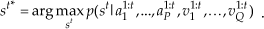
To perform recognition with the learned DDBN model, we can use a standard DBN inference algorithm to find label s^t, given the observations a_t^1:t,…,a^1:t_P,v_t^1:t,…,v_Q^1:t, by maximising p(s^t | a₁^1:t,…,a^1:t_P,v₁^1:t,…,v_Q^1:t) i.e.

s^{t *} = \arg \max_{s^{t}} p (s^{t} | a_{1}^{1 : t}, \dots, a_{P}^{1 : t}, v_{1}^{1 : t}, \dots, v_{Q}^{1 : t}) .

(11)

Given the input data D, the DDBN's topology learning algorithm for speech features and the speech recogniser is summarised as follows.

Algorithm:

Learning the audio block

For i=1,…until no improvement in the score of the estimated structure between audio input layer and acoustic features layer

1.1

Add one node into acoustic features layer;

1.2

Apply SEM to learn the structure using U_{_A}

Learning the visual block

For i=1, until no improvement in the score of the estimated structure between the visual input layer and the visual features layer;

2.1

Add one node into the visual features layer

2.2

Apply SEM to learn the structure using U__V

Inferring the values of H¹_{_A} and H¹_{_V}, according to the given data U_{_A}, U_{_V} and the learned structures in steps 1 and 2

Learning the cross-modality block

For i=1, until no improvement in the score of the estimated structure between the shared features layer and the single modality features layer;

4.1

Add one node into the shared features layer

4.2

Apply SEM to learn the structure using H₁ = {H¹_{_A}, H¹_{_V}}

Add the links between the label node and the shared feature nodes (this step is not necessary for isolated-word recognition)

Construct the transition network topology of the DDBN

Apply parameter EM to learn the parameters of the spatial network and transition network of the DDBN using D

Output the DDBN models

4. Experimental Setup and Results

In this section, we compare our DDBN model with a two-stream DBN model in [7] (as shown in Figure 7) and a widely used coupled HMM in [13] (as shown in Figure 8). Our experiments are conducted on Tibetan audio-visual speech classification of isolated letters, digits and command words.

Figure 7.

A two-stream DBN model for audio-visual speech recognition

Figure 8.

A coupled HMM model for audio-visual speech recognition

4.1 Datasets Description

5 male speakers say the digits 0 to 9 four times and 10 speakers (5 males and 5 females) say 30 Tibetan letters 4 times. In these cases the data were acquired using a laptop equipped with a webcam and microphone, so the digits and letters speech data are corrupted with environmental noise from classrooms and dormitories, much like the noise that a robot often encounters. 20 speakers (10 males and 10 females) say 10 command words in Tibetan three times. This data is made up of clean audio. These three datasets can be downloaded respectively from:

https://dl.dropbox.com/u/78851322/digits.rar

https://dl.dropbox.com/u/78851322/letters.rar

https://dl.dropbox.com/u/78851322/commandwords.rar

4.2 Data Pre-processing

The original audio signal is down-sampled to 8 KHz. Each observation frame has a 20ms window with 10ms overlaps. So the audio input to the DDBN comprises of 160 real-value nodes fed with 160 pieces of raw data, which is the normalised absolute value of amplitude of a speech signal in time domain. For two-stream DBN and coupled HMM models, the acoustic MFCCs features with 24-dimension are used as audio observation input.

For the video, we employ our facial point detection and tracking algorithm [14] to automatically detect and track 28 points. The 28 facial feature points are located around each facial component including eyes, nose and mouth, as shown in Figure 9(a). Given the detected 28 points, we can then extract the 8 points near the mouth as shown in Figure 9(b) in order to characterise mouth movement.

Figure 9.

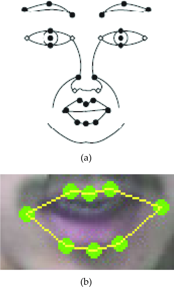
(a) Twenty eight facial feature points, and (b) the 8 facial feature points around the mouth

Accurately detecting and tracking these 28 facial feature points is challenging due to variation in facial expression, head orientation and illumination. In addition, facial hair such as a beard may occlude some facial points near the mouth. To address this challenge, we developed a hierarchical multi-modal and multi-state facial feature-tracking algorithm [14] that can robustly track the 28 points in real time. Our facial feature detection and tracking algorithm consists of two main steps; facial feature point detection and tracking. In the detection phase the face region is first detected by a non-parametric discriminative analysis (RNDA) face detector [15]. Based on the detected face region, a RNDA is further applied to detect two eye positions, as shown in Figure 10(a). The detected face and eye positions provide normalisation and initial localisation of the facial feature points, as shown in Figure 10(b). Then the initial facial feature point positions are further refined, whereby we employ pyramidal Gabor wavelets at different scales and orientations for facial feature point representation. Gabor wavelet based feature representation has the psychophysical basis of human vision and is more tolerant to variation in external illumination. Given the Gabor representation, facial point position refinement is performed by Gabor feature vector matching via a fast phase-based Gabor wavelet matching, as shown in Figure 10(c).

Figure 10.

Facial feature point detection. (a) face and eye detection, (b) initial facial feature point localisation, and (c) final detected facial feature points after refinement

In the tracking phase, given the detected 28 facial feature points, Kalman Filtering is used to model the dynamic of each facial feature point and to track feature points over time. To avoid tracking drift, the tracked facial feature positions are constrained by a pre-trained, hierarchical, multi-modal and multi-state shape model [14], which captures the spatial relationships among the facial feature points under different facial expressions and head poses. The shape model geometrically constrains the tracked facial points such that their spatial relationships must satisfy certain geometric constraints, therefore allowing all points to be tracked simultaneously and preventing individual points from drifting away under significant face pose or expression changes. Figure 11 shows examples of tracked facial feature points under different head poses and facial expressions.

Figure 11.

Facial feature point detection and tracking results under different head poses, facial hair, and facial expressions. The tracked points are marked in green and the red letter shows the head pose and facial expression.

Given the tracked 28 facial feature points, we then extract the 8 points near the mouth, as shown in Figure 9(b). From the 8 mouth points, we can compute the distance between left and right mouth corner as the width of mouth opening and the 3 distances between 3 points on the upper lip and 3 points on the lower lip as the heights of mouth opening, as shown in Figure 12. Owing to the different size of each speaker's face in videos (as shown in Figure 13), we take the differences of these four distances, in 2 contiguous video frames, as the input data of the previous frame. The video input data is processed at 20 Hz. Since the audio input data was processed at 8 KHz, the video input data was interpolated to make it occur at the same frame rate as the audio input data.

Figure 12.

The width and heights of a speaker's mouth opening

Figure 13.

Example video frames from 3 datasets

4.3 Recognition Results

Research with the articulator data [12] indicates that two factors are sufficient to represent the steady state of the articulators of the vowels. In this paper, we let each hidden feature node of the DDBN be a two dimensional vector of the hidden continuous state, which is adequate to group the acoustic and visual data into sub-words.

We combined the unlabelled audio and video data of letters, digits and command words for the DDBN's unsupervised feature learning (no test data was used for this process).

Table 1 shows the comparison results. It can be seen that our model shows a significant performance improvement over the results of a two-stream DBN and coupled HMM.

Table 1.

Experiment results on Tibetan audio-visual speech classification

	Digits	Letters	Words
DDBN	90.1%	98.2%	99.4%
two-stream DBN	64.4%	72.3%	96.2%
coupled HMM	62.3%	70.9%	95.4%

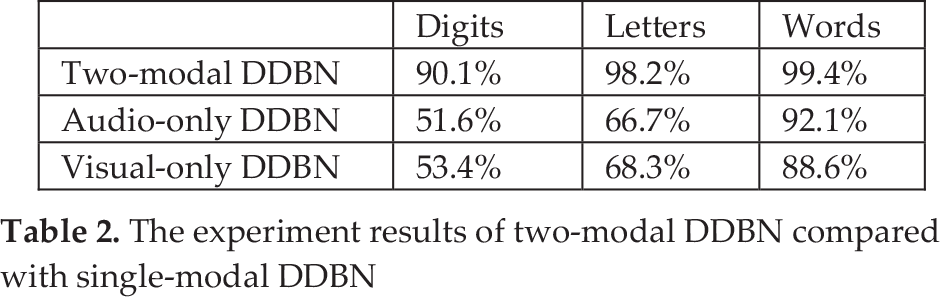
Also, we can compare our audio-visual DDBN with an audio-only DDBN (dynamic audio block) and a visual-only DDBN. The comparison results are shown in Table 2. It can be seen that our middle integration model shows a better result than other two single modality model for audio-visual speech data.

Table 2.

The experiment results of two-modal DDBN compared with single-modal DDBN

	Digits	Letters	Words
Two-modal DDBN	90.1%	98.2%	99.4%
Audio-only DDBN	51.6%	66.7%	92.1%
Visual-only DDBN	53.4%	68.3%	88.6%

5. Discussion

Speech remains the most natural mode of interaction between human and robot. Robust and accurate speech recognition is, therefore, important for successful human robot interactions. To this goal, we propose to learn a new feature representation (they can be acoustic features, visual features or multi-modal shared features) based on a DDBN from the raw speech data, in an unsupervised manner and without any prior knowledge. The recognition models based on the DDBN can capture the feature dependences both in space and time. The proposed feature learning method is effective for modelling high-dimensional multi-modal time series data.

In future works, we will investigate the optimal structure learning in a spatial network, including the number of hidden nodes and links. Although greedy learning of the number of nodes is simple and efficient, such an approach cannot guarantee an optimal solution, so we will investigate other spatial-temporal clustering methods to better determine the number of feature nodes.

Furthermore, the traditional EM algorithm we used improves the structure score in M-step through a greedy hill climbing procedure, which mutates the structure through adding, removing or reversing one link of the existing structure and finding the mutation with largest score. Although it is guaranteed to improve the structure score, the greedy search over the structure space can be easily trapped in a local optimum (and it is very “local”, as the structure space is huge). To address this problem, we will use an exact structure learning method as proposed in [16]. Future work will also include further validation of our method, including a comparison with other deep learning methods [17].

References

Gowdy

Subramanya

Bartels

Bilmes

(2004) DBN based multi-stream models for audio-visual speech recognition. In Proc. ICASSP: 993–996.

Zhang

Diao

Huang

Bartels

Bilmes

(2003) DBN based multi-stream models for speech. In Proc. ICASSP.

Sun

A L

Jiang

D M

Liu

G Y

Hichem

Werner

(2007) Research on DBN-based continuous speech recognition and phoneme segment. In Application Research of Computers, 24: 104–106.

Nefian

Liang

L H

X B

(2002) A coupled HMM for audio-visual speech recognition. In Int'l Conf Acoustics, Speech and Signal Processing: 2013–2016.

Dahl

G E

Ranzato

M A

Mohamed

A R

Hinton

(2010) Phone Recognition with the Mean-Covariance Restricted Boltzmann Machine. In Advances in Neural Information Processing Systems: 469–477.

Lee

Largman

Pham

A Y

(2009) Unsupervised Feature Learning for Audio Classification Using Convolutional Deep Belief Networks. In Advances in Neural Information Processing Systems: 1096–1104.

Saenko

Livescu

(2006) An Asynchronous DBN for Audio-visual Speech Recognition. In Spoken Language Technology Workshop: 154–157.

Murphy

K P

(2002) Dynamic Bayesian Networks: Representation, Inference and Learning. PHD Thesis. University of California, Berkeley.

Zheng

Y L

Hasegawa-Johnson

(2003) Acoustic Segmentation Using Switching State Kalman filter. In IEEE International Conference on Acoustics, Speech, and Signal Processing: I-752–I-755.

10.

Fridman

(1998) The Bayesian Structural EM Algorithm. In Conf. on Uncert. in AI: 129–138.

11.

Dempster

Larid

Rubin

(1997) Maximum likelihood from incomplete data via the EM algorithm. In Journal of the Royal Statistical Society: 39:1–38.

12.

Harshman

Ladefoged

Goldstein

(1977) Factor analysis of tongue shapes. In JASA, 62(3): 693–707.

13.

Brand

Oliver

Pentland

(1997) Coupled hidden Markov models for complex action recognition. In IEEE International Conference on Computer Vision and Pattern Recognition: 994–999.

14.

Wang

(2005) Learning Discriminant Features for Multi-View Face and Eye Detection. In: CVPR.

15.

Tong

Wang

Zhu

(2007) Robust facial feature tracking under varying face pose and facial expression. In Pattern Recognition, 40: 3195–3208.

16.

Campos

C P

Zeng

(2011) Efficient Structure Learning of Bayesian Networks using Constraints. In Journal of Machine Learning Research, 12:663–689.

17.

Ngiam

Khosla1

Kim

M Y

Nam

Lee

A Y

(2011) Multimodal deep learning. In ICML: 689–696.