
Abstract
This paper describes a novel self-occlusion detection approach for depth image using SVM. This work is distinguished by three contributions. The first contribution is the introduction of a new self-occlusion detection idea, which takes the self-occlusion as a classification problem for the first time, thus the accuracy of the detection result is improved. The second contribution is two new self-occlusion-related features, named maximal depth difference and included angle. The third contribution is a specific self-occlusion detection algorithm. Experimental results not only show that the proposed approach is feasible and effective, but also show that our works produce better results than those previously published.
Keywords
1. Introduction
Self-occlusion means that, from a certain viewpoint, one part of an object is occluded by another part. There are self-occlusion problems in most visual tasks, such as object recognition, motion tracking, 3D reconstruction, robot grasping, environmental perception and assembling, etc. [1–3]. Self-occlusion will affect the results of recognition, tracking, reconstruction and other visual tasks. Therefore, how to detect self-occlusion accurately is one of the problems that must be solved in the visual domain.
As an important research topic in computer vision, more and more scholars have paid attention to self-occlusion detection. Castellani [4] detected self-occlusion by establishing a foreground-background relation between neighbouring regions of a visual object. However, this method is limited to objects with simple shape. Adopting the threshold method, Park [5] separated the self-occlusion region from the depth image enhanced by a median filter, yet this method is limited to the case of single self-occlusion, so is not suitable for an object with multiple self-occlusion. Schmaltz [6] overcame typical silhouette ambiguities caused by self-occlusion through tracking each part of an object, rather than the whole object, aiming to avoid self-occlusion, but not to detect self-occlusion. Christoudias [7] solved self-occlusion problems using a multiple camera system. However, this method involves high costs, large equipment, installation problems and other shortcomings, making the method difficult to use widely. Gay-Bellile [8] presented a self-occlusion modelling framework during image-based non-rigid registration, but did not give a concrete method to detect self-occlusion. Lee [9] used a shape conversion matrix to solve the point correspondence errors caused by self-occlusion. Unfortunately no practical self-occlusion detection method is provided. Pizarro [10] detected self-occlusion in an object image using the FFD (Free-Form Deformations) warp computed from wide-baseline point matches between a template and an object image. However, this method is template-based, so is not suitable for an unknown object.
To solve the above problems, in 2010 and 2011, we sought the solution to self-occlusion detection based on the mean curvature and average depth difference of a depth image respectively [11,12]. In [11] the features, such as mean curvature, curvature threshold and depth threshold, are adopted to detect the self-occlusion. In [12] we detected the self-occlusion successfully by using the average depth difference and its threshold. But the thresholds in these two methods vary with depth image. In other words, the general method for selecting a threshold has not been found yet. So the methods have limitations and at the same time, the accuracy of the self-occlusion detection result still needs to be improved.
In order to overcome the deficiencies of the existing methods, this paper proposes a novel self-occlusion detection approach based on machine learning idea. Utilizing the maximal depth difference feature and included angle feature of depth image creatively, the approach accomplishes self-occlusion detection by training a support vector machine. The experiment results show that the proposed approach not only has better generality, but also has higher accuracy.
The rest of the paper is organized as follows. Section 2 describes the depth image and its two new self-occlusion-related features. Section 3 explains the details of our proposed approach. Section 4 presents our experiment results and section 5 concludes the paper.
2. Depth image and its two new self-occlusion-related features
2.1 Depth image
A depth image is a kind of image with a special form. It complies with the basal image format, which is an array of pixels organized as rows and columns. The main difference between depth images and grey images is the meaning of pixel. For grey images, the pixel value represents greyscale or photosensitive strength. For depth images, the pixel value represents the distance to the reference plane. A depth image directly reflects the three-dimensional geometric information of the scene surface and has advantages such as high accuracy and is not affected by illumination, shadow or other factors. Therefore, visual systems based on depth image information are increasingly an area of interest.
Recently, we have found two new self-occlusion-related features in depth images, named maximal depth difference feature and included angle feature. The following paragraphs will introduce them.
2.2 Maximal depth difference feature
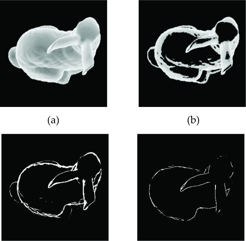
The depth difference reflects the depth relationship between the points in the depth image. For each self-occlusion point in a self-occlusion region of a depth image, there is at least one neighbour that has quite a large depth discontinuity from it, so depth difference can be used to detect self-occlusion. Maximal depth difference feature refers to the maximum of the depth differences between any pixel and its eight neighbours in a depth image. Fig. 1 shows a Bunny's depth image and the corresponding maximal depth difference map. From Fig. 1 we can tell that the bigger the maximal depth difference of a pixel is, the more likely it is a self-Compared with the average depth difference feature proposed in [12], the advantage of the maximal depth difference feature is that it not only considers the relationship between the depth difference and self-occlusion, but also strengthens the effect of the depth difference feature on detection of a result. For example, for a self-occlusion point in a depth image, if only one neighbour has a bigger depth difference with it, then the average depth difference feature will weaken the effect of depth difference. In this case, this self-occlusion point will be mistaken as a non-self-occlusion point because of its smaller average depth difference. As a result, the detection accuracy will be reduced. However, the maximal depth difference feature can maximize the effect of the depth difference feature on detection of a result and therefore improve the detection accuracy.

A Bunny's depth image and maximal depth difference map; (a) Depth image of a Bunny (b) Maximal depth difference map of a Bunny with depth scale
2.3 Included angle feature
For each pixel in a depth image, we can get a corresponding three-dimensional coordinate in a three-dimensional space. Under the constraint of the 8-neighbourhood model, each pixel in a depth image can form eight vectors with its eight neighbours by using their corresponding three-dimensional coordinates. There is a vector angle between each vector and the camera direction vector. Thus, there are eight vector angles for each pixel. The included angle feature of each pixel refers to the minimal angle among its eight vector angles. Fig. 2 shows the sketch maps of the included angle feature obtained from the Bunny's depth image. In Fig. 2(a) the included angle feature values for all pixels are shown. Fig. 2(b) shows the pixels whose included angle feature values are smaller than 45°. Fig. 2(c) shows the pixels whose included angle feature values are smaller than 22.5°. Fig. 2(d) shows the pixels whose included angle feature values are smaller than 10°. From Fig. 2 we can know, in a depth image, the smaller the included angle feature value of a pixel is, the more likely it is a self-occlusion point. Therefore, included angle features can also be used as an important basis for detecting the self-occlusion phenomenon. In general, we calculate included angle features in the camera coordinate system by default.
The sketch map of a Bunny's included angle feature; (a) All pixels (b) Pixels with feature value smaller than 45° (c) Pixels with feature value smaller than 22.5° (d) Pixels with feature value smaller than 10°
3. Self-occlusion detection approach
3.1 Problem statement and overall idea of proposed approach
The aim of self-occlusion detection is to locate a self-occlusion boundary in the depth image of a visual object, as shown in Fig. 3. In Fig. 3(a), an ideal visual object is composed of a triangle ABC and a quadrangle BCDE. In current view, the quadrangle BCDE is occluded by the triangle ABC and the occluded region is triangle A'BC. AB and AC, which corresponds to the two red lines of the depth image in Fig. 3(b), are the two edges where the self-occlusion phenomenon occurs. The purpose of self-occlusion detection is to find and mark all the pixels that form the two red lines in Fig. 3(b).
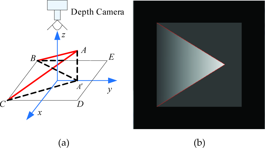
The sketch map of self-occlusion detection; (a) An ideal visual object; (b) The depth image of visual object and its self-occlusion boundary
After deciding to use the maximal depth difference feature and included angle feature for detecting the self-occlusion phenomenon, the overall idea of the proposed self-occlusion detection approach can be described as follows. First, obtain positive and negative samples from the sample collection data source and use their normalized feature values to train support vector machine (SVM). Then the SVM model for detecting self-occlusion can be gained. Second, traverse the depth image to be detected. In this step, each pixel in the depth image is treated as a test sample, then the maximal depth difference feature and included angle feature of each sample are calculated. After that, the feature vector of each sample is formed by normalizing and combining its feature values. Finally, the trained SVM model is used for predicting each sample, to get the final self-occlusion detection result. Fig. 4 shows the overall process of the proposed self-occlusion detection approach. More details are described in the following sections.

The overall process of the proposed self-occlusion detection approach
3.2 Feature extraction
Maximal depth difference feature and included angle feature have been described in Section 2. The extraction methods of these two features are given in the following.
3.2.1 Extracting the maximal depth difference feature
Suppose that the coordinate of a pixel in a depth image is (i,j) and the depth of the pixel is depth(i,j). Then the coordinates of its eight neighbours are (i − 1, j − 1), (i, j −1), (i + 1, j − 1), (i − 1,j), (i + 1, j), (i − 1, j + 1), (i, j + 1) and (i + 1, j + 1) respectively and the depth of the neighbours are depth(i − 1, j − 1), depth(i, j − 1), depth(i + 1, j − 1), depth(i −1,j), depth(i + 1, j), depth(i − 1, j + 1), depth(i, j + 1) and depth(i + 1, j + 1) respectively. The maximal depth difference feature of pixel (i, j) is defined as
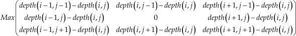
The method for extracting the maximal depth difference feature of a depth image can be described as follows. Traverse all the pixels in the depth image. If the current pixel is a background point or visual object boundary point, then 0 is assigned to its maximal depth difference feature. If the current pixel is a visual object internal point, its corresponding feature value is calculated with Eq. (1). Thus, the feature matrix of maximal depth difference can be obtained after the whole depth image is traversed.
3.2.2 Extracting the included angle feature
In a depth image, the vectors formed by the three-dimensional coordinates of pixel (i, j) and its eight neighbours are denoted by Vi−1, j−1, Vi, j−1, Vi+1, j−1, Vi−1, j, Vi+1, j, Vi −1, j+1, Vi,j+1 and Vi+1,j+1 respectively. The included angles formed by eight vectors and the camera direction vector are denoted by

respectively. Then the included angle feature of pixel (i, j) can be defined as

The method for extracting the included angle feature of a depth image is described as follows. First, obtain the three-dimensional coordinate of each pixel in the depth image. Second, traverse all the pixels in the depth image. If the current pixel is a background point or visual object boundary point, then π is assigned to its included angle feature. If the current pixel is a visual object internal point, its corresponding feature value is calculated with Eq. (2). Finally, the feature matrix of the included angle can be obtained, after the whole depth image is traversed.
3.3 Selection of positive and negative samples
In this paper, self-occlusion is detected by using SVM. As the SVM is a kind of supervised machine learning method, we should mark the pixels in the depth image as positive and negative samples before training the SVM. The method for selecting positive and negative samples is described as follows.
Extract the maximal depth difference feature and included angle feature of each pixel in the depth image.
Set up some pairs of thresholds manually. Each pair of thresholds, which consists of the maximal depth difference feature and the included angle feature, is used to mark all the pixels in the depth image respectively. During the marking process, the pixel whose maximal depth difference feature value is bigger than the depth threshold and whose included angle feature value is smaller than the angle threshold is marked as positive sample, namely the self-occlusion point. Otherwise, the pixel is marked as a negative sample, namely a non-self-occlusion point. If the number of marked positive samples is almost the same as the actual existent number of self-occlusion points in the depth image, then the pair of thresholds is recorded. Otherwise it is discarded.
Calculate the average of all the recorded thresholds as the final thresholds. This pair of thresholds is utilized to mark all the pixels in the depth image again. Then the final positive and negative samples for training the SVM are obtained.
3.4 Training SVM and self-occlusion detection
After obtaining the final positive and negative samples, as the two kinds of features proposed in this paper are in different scale, to reduce the influence of features with a different scale on training result, the values of the two features must be normalized before training the SVM. The normalization method is as follows. First, obtain the maximum of the maximal depth difference feature by traversing the obtained maximal depth difference feature matrix and assign π to the maximum of the included angle feature. Then, normalize the maximal depth difference feature and the included angle feature by the maximum and minimum normalization method. On this basis, the two kinds of normalization features of positive and negative samples are combined to train the SVM, thus a classifier for self-occlusion detection can be obtained.
Once the SVM is trained, the next step is using the trained SVM to detect self-occlusion points in the depth image. The specific steps are as follows. First, each pixel in the depth image is regarded as a test sample, the maximal depth difference feature and the included angle feature of each sample are extracted. Then the feature values of each sample are normalized and combined into a feature vector. Second, take the feature vector of each pixel as the input of the SVM to detect self-occlusion. In this process, the trained SVM is used to mark each pixel as a positive or negative sample. Thus, the final self-occlusion detection result can be obtained after the whole depth image is traversed.
3.5 Description of the self-occlusion detection algorithm
The proposed self-occlusion detection algorithm is described as follows.
4. Experiment and analysis
4.1 Experiment scheme and self-occlusion detection results
To validate the effect of the proposed approach, we tested our approach using the depth images in the Stuttgart Range Image Database on http://range.informatik.unistuttgart.de/htdocs/html. The hardware for the experiment is a computer equipped with CPU of Pentium(R) Dual-Core 2.93GHz and 2.0G memory. The self-occlusion detection program is implemented by C++. The SVM is C-SVC, the penalty factor for SVM is 50 and the decision function is linear kernel function.
We take the Bunny's image in Fig. 1 as the data source for extracting the training sample. In order to divide the samples into positive and negative ones, we record 6 pairs of thresholds (shown in Table 1). Each pair of thresholds consists of a depth threshold and an angle threshold. We take the average (5.48796, 14.49°) of the 6 pairs of thresholds in Table 1 as the final thresholds for distinguishing positive and negative samples.
The thresholds for dividing samples
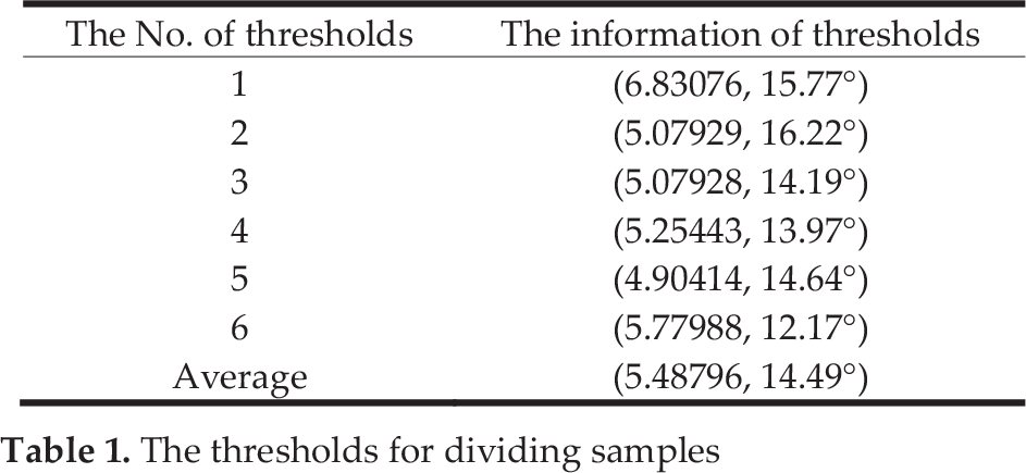
According to the final thresholds (5.48796, 14.49°), the pixels in the Bunny's depth image can reasonably be divided into positive and negative samples. In our experiment 1205 positive samples and 158,795 negative samples were obtained. The ratio of positive to negative samples is about 1:132. Considering the effect of the ratio and the distribution of positive and negative samples on training the SVM, we then decided to use another pair of thresholds (1.22604, 24.11°) to select final training samples from the obtained samples. In this pair of thresholds, the depth threshold is smaller than 5.48796 and the angle threshold is bigger than 14.49°. Therefore, it can ensure that not only all the positive samples can be selected, but also the large number of negative samples, which have little influence on classification, can't be selected. Thus, the final positive and negative samples suitable for training the SVM can be obtained.
Based on the idea above, 1205 positive samples and 3441 negative samples were selected for training the SVM. After training the SVM, 5 support vectors are obtained. Two of them are from positive samples and the others are from negative samples. On this basis, we perform self-occlusion detection on different depth images using the trained SVM (part of our detection results are shown in Fig. 5). For each group of images in Fig. 5, the left is the original depth image and the right is the corresponding self-occlusion detection result. The pixels marked as red in the result images are the self-occlusion points. From Fig. 5 we know the proposed approach can detect the self-occlusion phenomenon correctly.

The different depth images and their self-occlusion detection results
In addition, Table 2 shows the time-consumption of the proposed approach for detecting different depth images. The time-consumption for each depth image is the average value of ten times the experiment results. From Table 2, we can tell that most of the time is consumed by feature extraction, while less time is consumed by using the SVM to detect self-occlusion. On average, a 400*400 depth image can undergo self-occlusion detection in 0.19377 seconds by the proposed approach, under our experiment conditions.
The time-consumption of self-occlusion detection for different depth images


4.2 Experiment comparison and analysis
To evaluate the performance of the proposed self-occlusion detection approach more reasonably, we compare it with an existing self-occlusion detection method. Until now, most published papers related to self-occlusion have not given a specific self-occlusion algorithm and experimental results. Therefore, we compare the proposed approach with the method proposed in [12], which is our latest published research. To obtain the quantitative evaluation for the proposed method, we also need ground truth as the criteria for self-occlusion detection. However, as far as we know, scholars generally verify the self-occlusion detection results by visual observation, so the ground truth for self-occlusion detection of depth images does not yet exist. Therefore, we have generated some ground truths. The generating method is as follows. First, the positive sample extraction method proposed in 4.1 is adopted to deal with the depth image and the obtained positive samples are marked as the self-occlusion pixels. After that, a temporary result can be generated. Then, the temporary result is optimized manually by visual observation until all the self-occlusion pixels are marked. Thus, the ground truth of the depth image is obtained. The comparative results of the method in [12] and the proposed approach are shown in Fig. 6. Fig. 6(a) shows depth images for detecting, Fig. 6(b) shows the ground truth, Fig. 6(c) shows the self-occlusion detection results of the method in [12] and Fig. 6(d) shows the detection results of the proposed approach in this paper.

The comparison of self-occlusion detection results between the method in [12] and the proposed approach
As can be seen from Fig. 6, the method in [12] can detect most self-occlusion regions, however the accuracy of the detection results is lower, which is mainly embodied in two aspects. Firstly, it detects less self-occlusion boundaries compared with the proposed approach. Secondly, some self-occlusion boundaries are not continuous. This is because the average depth difference weakens the effect of the depth difference feature on self-occlusion detection. As a result, some self-occlusion points can't be detected successfully. In fact, a point in a depth image can be regarded as a self-occlusion point as long as one of its eight neighbours has a bigger depth difference with it. Meanwhile, for the method in [12], the depth threshold should be set manually before detecting. That is, the depth threshold should be recalculated according to different images. Therefore, the generality of the method is reduced. In contrast, by using the maximal depth difference feature and included angle feature, the effect of depth difference is maximized and more valuable information in the depth image is utilized for detecting self-occlusion, thus the self-occlusion detection results of the proposed approach are better. Namely, more self-occlusion boundaries are detected, which is more like the actual situation. At the same time, the self-occlusion points on occlusion boundaries are more continuous. In addition, the proposed approach based on machine learning has better generality, that is to say, once the SVM is trained, it can suit any depth image.
In order to quantitatively evaluate the proposed approach, Table 3 shows the statistical analysis of the self-occlusion detection results obtained from different methods. In Table 3, Nstandard is the number of the self-occlusion pixels in ground truth, Ndetected is the number of self-occlusion pixels in detection results and Nmatched is the number of the self-occlusion pixels in detection results that match the self-occlusion pixels in ground truth. The recognition rate Nmatched/Nstandard and the error rate (Ndetected − N matche d )/Ndetected are taken as the performance metric to decide which method is quantitatively better.
Statistical analysis of the self-occlusion detection results

From Table 3, we can see the error rate of the proposed approach is slightly higher than that of the method in [12], but the recognition rate of the proposed approach is much higher than that of the method in [12], that is to say, the detection result of the proposed approach is closer to the ground truth. Therefore, the proposed approach is quantitatively better.
5. Conclusions
A self-occlusion detection approach based on machine learning idea is proposed. At first, the maximal depth difference feature and included angle feature are extracted to train the SVM. Then the trained SVM is used to detect the self-occlusion phenomenon in a depth image. The proposed approach has the following advantages.
The approach takes the self-occlusion detection as a classification problem for the first time, namely, we study self-occlusion based on the idea of machine learning, and better results are achieved.
Two new self-occlusion-related features named maximal depth difference and included angle are proposed, and they are successfully used to detect the self-occlusion phenomenon.
Compared with existing methods, the proposed approach not only can detect the self-occlusion phenomenon efficiently and accurately, but also has generality.
Footnotes
6. Acknowledgments
This work is supported by State Key Laboratory of Robotics and Systems (HIT) under Grant No. SKLRS-2010-ZD-08, National Natural Science Foundation of China under Grant No. 60975062 and Natural Science Foundation of Hebei province under Grant No. F2010001276.