New Method for Tuning Robust Controllers Applied to Robot Manipulators

Abstract

This paper presents a methodology to select the parameters of a nonlinear controller using Linear Matrix Inequalities (LMI). The controller is applied to a robotic manipulator to improve its robustness. This type of dynamic system enables the robust control law to be applied because it largely depends on the mathematical model of the system; however, in most cases it is impossible to be completely precise. The discrepancy between the dynamic behaviour of the robot and its mathematical model is taken into account by including a nonlinear term that represents the model's uncertainty. The controller's parameters are selected with two purposes: to guarantee the asymptotic stability of the closed-loop system while taking into account the uncertainty, and to increase its robustness margin. The results are validated with numerical simulations for a particular case study; these are then compared with previously published results to prove a better controller performance.

1. Introduction

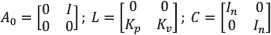
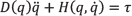
Rigid robots are dynamic systems that have multiple applications in industry, including welding, painting, and assembly of electronic parts. Additionally, robot manipulators can be used either in jobs where human life may be at risk or in processes that require a very high production rate. These numerous applications lead to the development of analytical tools to ensure better performance of the electromechanical systems. There are many research works in this field; for example, the problem of the robot's positioning [1] is a well-researched one in robotics, that is, the way in which its coordinates change. This is a relevant problem because robots are often used to move objects from one point to another. To address this problem, different control strategies using a mathematical model of the manipulator robot have been proposed. This mathematical model can always be represented as follows:

$D\left(q\right)\ddot{q}+H\left(q,\dot{q}\right)=\tau \mathrm{ }$

(1)

where

$H\left(q,\dot{q}\right)=V\left(q,\dot{q}\right)+W\left(\dot{q}\right)+U\left(q\right)$

(2)

D(q)^n×n is a positive definite matrix for all values of q and is called the inertia matrix; V(q,q̇)^n×1 is the vector that characterizes the centrifugal and Coriolis forces that appear on the manipulator; W(q̇)^n×1 is the friction forces vector and U(q)^n×1 the vector that represents the gravitational forces; q represents the generalized coordinates vector, i.e., the angular position for the rotating joints or the linear position for the prismatic (Cartesian) joints; τ is the action that produces the movement of the robot which, for rotating joints, represents the torque produced by the movement of the robot and is called control torque. It is important to mention that most of the methods used to calculate the control law for robot manipulators explicitly use their mathematical model. However, in practice, it is not possible to obtain a mathematical model that accurately represents the robot's dynamic behaviour. This in turn causes a mismatch between the practical results and the ones obtained with the mathematical model. This problem has been considered by several authors, including [2], [3], [4] and [5], where the main idea was to achieve robustness of the control system for the manipulator robot. Techniques used to achieve this objective include adaptive control and nonlinear robust control. In [4] a control algorithm is proposed based on exact linearization in the sense of [6] using the robot dynamics equation. When this technique is employed, a linear model is obtained and a state feedback is then applied to guarantee the stability of the linear system; next, a robust compensation is added to reduce the effects of the modelling errors. This compensation is designed using the variable structure theory. Modelling errors are treated as unstructured uncertainty in the inertia matrix as well as in the centrifugal and Coriolis forces; this type of compensation is discussed in [5]. In [2], a control law that guarantees robustness in the dynamic system under the condition that the mathematical model satisfies the condition of linearity on the parameters is presented. This control law is modified in [3] to improve the results. A robustness analysis is presented in [7], where a decoupled multivariable PID controller was proposed for the linearized model, obtaining a system of linear differential equations with matrix coefficients expressed in terms of the parameters of the PID controller and the inertia matrix evaluated at the reference point. This approach permits the application of Kharitonov's theorem (see [8]) to ensure robust stability; however, the type of uncertainty considered leads to very conservative results. A compendium of papers related to robust control of robot manipulators can be found in [9]. Robust control techniques applied to robot manipulators have recently been discussed in various publications; for example, in [22] an output feedback sliding mode robust control method was proposed, using the Lyapunov method to establish semi-global stability conditions. [23] proposes a neural network control algorithm based on H_∞ theory, where the controller designed does not need a precise model of the robot. The interesting results of designing an image-based robust feedback controller to compensate parametric uncertainty are presented in [24]. In [10] the authors present an interesting application for the agricultural sector, where a mechanical structure used to harvest watermelons was redesigned to take the form of a manipulator robot. This mechanical system was controlled applying robust control techniques based on gain schedule and μ-synthesis, and its main achievement was to attain cost reductions. In [11] a robust adaptive control technique based on Lyapunov theory is presented to guarantee convergence in the trajectory tracking of a pair of coordinated robots that perform tasks together. Here, not only the coupled dynamics of the two robots but also the dynamic and parametric uncertainty of the control system is taken into account. Other robust control strategies based on fuzzy systems are applied to holonomic and non-holonomic systems in [12], where robustness conditions are obtained while taking both parametric uncertainty and external disturbances in the control system into account; other important results related to this topic are presented in [20] and [21], where a fuzzy logic controller is designed to solve the problem of output regulation in a servomechanism with nonlinear backlash. Results on PD controller tuning for rigid robots, taking into account the dynamics of the actuators (DC motors), are presented in [13], showing improvements on previous results.

1.1 Main contribution

From the section above it may be seen that there are a variety of means to solve the robust control problem in robot manipulators; this work, unlike others, proposes a method based on LMI to select the controller parameters to improve its capability to tolerate the uncertainty of the mathematical model of the manipulator robot. The main result consists in the proper selection of the parameters of a nonlinear controller that heavily relies on the mathematical model of the robot to improve the robustness margin of the closed-loop control system. Firstly, an exact linearization control law is applied, and then the problem is stated as a pole placement control problem for a linear system with dynamics uncertainty. Here, the key point is to properly choose the multivariable state feedback so that the robustness margin is improved. This is achieved by using the Matlab toolboxes software. The aim is to improve the robustness margin through proper allocation of the closed-loop poles of the linear system, thereby compensating for the uncertainty of the mathematical model; previous results are merely based on applying high-gain controllers. The effectiveness of the control law proposed in this work is shown through a series of simulations which are compared with previous results shown in [19].

This paper is organized as follows: Section 2 shows preliminary results required in order to understand the outcome of this research; then, the automatic control problem of the manipulator robot is formulated in Section 3. Next, in Section 4, the main result is presented. Section 5 displays some simulations for the case of a planar robot with two degrees of freedom, and the results are compared to those previously published. Finally, in Section 6, the conclusions of this research work are presented.

2. Mathematical preliminaries

This paper has its basis in the method presented in [14], which verifies the robust stability property for a class of perturbed nonlinear systems with the following structure:

$\dot{x}=f\left(x\right)+g\left(x\right)$

(3)

where x ∈ Rⁿ, f(x) and g(x) are functions that belong to a vector field. In Equation (3) the nominal system is

$\dot{x}=f\left(x\right)\left(x\right)$

(4)

and g(x) is a nonlinear perturbation of the nominal system that satisfies the Lipschitz condition:

$||g\left(x\right)||\le \gamma ||x||\left(x\right)$

(5)

It is evident that the above condition prevents the equilibrium point of the nominal system from being modified while uncertainty is present. The method assumes that the equilibrium point of the nominal system (which may be, without loss of generality, x = 0) is exponentially stable; this implies that a Lyapunov function V(x) exists and that it satisfies the following conditions:

$c_1{||x||}^2\le V\left(x\right)\le c_2{||x||}^2\left(x\right)$

(6)

$\frac{\partial V\left(x\right)}{\partial x}f\left(x\right)\le -c_3{||x||}^2\left(x\right)$

(7)

$||\frac{\partial V\left(x\right)}{\partial x}||\le c_4{||x||}^2\left(x\right)$

(8)

The following lemma gives sufficient conditions to verify the robust stability of the perturbed system (3) (see [14]).

Lemma 2.1. Let x = 0 be an exponentially stable equilibrium point of the nominal system (4). Let V(x) be a Lyapunov function of the nominal system that satisfies (6)-(8). Assume that the perturbation g(x) satisfies (5). Then, x = 0 is an exponentially stable equilibrium point of the perturbed system (3). Furthermore, if all assumptions are globally valid, then x = 0 is globally exponentially stable.

This could be particularly relevant with a nominal linear time invariant system with a nonlinear perturbation such as the following:

$\dot{x}=Ax+g\left(x\right)\mathrm{ }\left(x\right)$

(9)

In this case, the equilibrium point x = 0 is exponentially stable if A is a Hurwitz matrix and the perturbation g(x) satisfies the following conditions:

$||g\left(x\right)||\le \frac{{\lambda }_{min}\left(Q\right)}{{2\lambda }_{max}\left(P\right)}||x||=\gamma ||x||\left(x\right)$

(10)

where λ_min(Q) and λ_max(Q) are the minimum and maximum eigenvalues of the matrices Q and P, respectively. These matrices are positive definite and satisfy the Lyapunov equation:

$PA+A^{T}P=-Q\left(x\right)$

(11)

In this case, the Lyapunov function is defined as V(x) = x^T Px and it is clear that it satisfies the conditions (6)-(8). Note that in (10), the parameter γ of Equation (5) is susceptible to be modified (to increase), since it depends directly on the eigenvalues of the matrices Q and P, which can take different values under the condition that they are positive definite. Moreover, it is possible to note that an increase in the parameter γ would lead to an increase in the maximum bound that must satisfy the nonlinear perturbation, and this in turn causes an increase in the robustness margin of the dynamical system. This opportunity to improve the robustness margin is the main motivation for this research work, however, unlike in [14], the problem here is stated as a convex optimization problem with respect to the parameter γ, which is solved using convex optimization techniques based on LMI.

3. Problem statement

The mathematical model of the manipulator robot that will be considered in this work is the one presented in Equation (1), where τ is assumed to be the control law, which is defined as follows:

$\tau ={\tau }_{ff}+{\tau }_{fb}\left(x\right)$

(12)

${\tau }_{ff}=H_0(q,\dot{q})\mathrm{ }\left(x\right)$

(13)

${\tau }_{fb}=D_0\left(q\right)\left[-K_{p}q-K_v\dot{q}\right]\left(x\right)$

(14)

where τ_ff represents the feedforward term and τ_fb is the feedback term of the control law. D₀(q) and H₀(q, q̇) are the nominal values of the inertia matrix and the vector of centrifugal, Coriolis, friction and gravity forces. These differ from the real values of the robot manipulators, which is why they are defined in a different way.

It is important to mention that the controller's parameters are the matrices K_p and K_v, and they form part of the feedback of the control law. Substituting the control law (12) into the manipulator model (1) the following equation is obtained:

$\ddot{q}=D^{-1}\left(q\right)\left[-K_{p}q-K_v\dot{q}\right]+f\left(q,\dot{q}\right)+p(q,\dot{q})\mathrm{ }\left(x\right)$

(15)

where

$f\left(q,\dot{q}\right)=D^{-1}\left(q\right)\Delta H\left(q,\dot{q}\right)\left(x\right)$

(16)

$\Delta H\left(q,\dot{q}\right)=H_0\left(q,\dot{q}\right)-H\left(q,\dot{q}\right)\left(x\right)$

(17)

$p\left(q,\dot{q}\right)=\left(D^{-1}\left(q\right)D_0\left(q\right)-I\right)\left(K_{p}q-K_v\dot{q}\right)\left(x\right)$

(18)

Now, with the following definition:

$x=\left[\begin{array}{c}{x}_1\\ x_2\end{array}\right]=\left[\begin{array}{c}q\\ \dot{q}\end{array}\right]$

(19)

the following representation of the robot in closed loop is obtained:

$\dot{x}=A_{c}x+g\left(x\right)$

(20)

Where:

$A_c={\left[\begin{array}{cc}0& I^{n\times n}\\ -K_p^{n\times n}& -K_v^{n\times n}\end{array}\right]}^{2n\times 2n}$

(21)

$g\left(x\right)=f\left(x\right)+p\left(x\right)$

(22)

It is clear that when the control law (12) is applied to the dynamic model of the manipulator robot, an equation of the form (3) is obtained, making it possible to apply the results from Lemma 2.1 in order to ensure the asymptotic stability property in the manipulator's control system; however, as mentioned in Section 2, the parameters K_p and K_v of the control law can be selected so that the upper bound of the nonlinear perturbation (10) increases, thereby increasing the robustness margin of the control system. Hence, the problem can be stated as follows:

Given the dynamic system represented by the following equation:

$\dot{x}=\left[\begin{array}{cc}0& I\\ -K_p& -K_v\end{array}\right]x+g\left(x\right)$

(23)

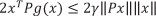
The matrices K_p and K_v are selected so that the control system represented by the Equation (23) is asymptotically stable and additionally maximizes the parameter y to satisfy the following condition:

$||g\left(x\right)||\le \gamma ||x||$

(24)

4. Main result

The main result of this work is based on Lemma 2.1, it is therefore necessary to establish the conditions that satisfy Equation (22). From the definition of g(x) the following condition can be obtained:

$||g\left(x\right)||=||f\left(x\right)+p\left(x\right)||\le ||f\left(x\right)||+||p\left(x\right)||$

(25)

Since matrix D(q) is a positive definite matrix, the following condition can be guaranteed (see [15], [16]):

$||D^{-1}\left(q\right)||\le k_1$

(26)

Therefore, we have:

$||f\left(x\right)||\le k_1||\Delta H(q,\dot{q})||$

(27)

Now, assuming that the uncertainty between the vectors H₀(x) and H(x) is upper bounded, and that in the equilibrium point (x = 0) both vectors have the same value, the following inequality is obtained:

$||\Delta H\left(q,\dot{q}\right)||\le k_2||x||$

(28)

resulting in the following condition:

$||f\left(x\right)||\le {k_{1}k}_2||x||={\eta }_1||x||$

(29)

On the other hand, the inertia matrix D(q) is a positive definite matrix that is lower and upper bounded by positive definite matrices. Additionally, the controller's matrices K_p and K_v require bounded elements to guarantee the Hurwitz property in matrix A_c; hence, it is always possible to obtain the following relation (see [9]):

$p\left(x\right)\le ||D^{-1}\left(q\right)D_0\left(q\right)-I||||K_{p}q-K_v\dot{q}\mathrm{ }||$

(30)

$p\left(x\right)\le {\alpha }_1||K_{p}q-K_v\dot{q}\mathrm{ }||$

(31)

$p\left(x\right)\le {\alpha }_1{\alpha }_2||x||$

(32)

$p\left(x\right)={\eta }_2||x||$

(33)

Therefore:

$||g\left(x\right)||\le {\eta }_1||x||+{\eta }_2||x||\le \gamma ||x||$

(34)

This condition allows us to apply the result presented in Lemma 2.1 to the case of the robotic manipulator dynamic system. As mentioned earlier, in Equation (10) it can be noted that it is possible to increase the upper bound by appropriate selection of the matrices K_p and K_v, which in turn will increase the ability of the robot manipulator closed-loop system to support greater uncertainty. To do this, a search procedure based on LMI is performed. This procedure is based on the results presented in [17], for which the following theorem and corollary are now presented.

Theorem 4.1. Considering system (23), the equilibrium point (x = 0) is asymptotically stable if the following matrix inequality is satisfied:

$P{A}_c+A_c^{T}P+{\gamma }^{2}PP+I<0$

(35)

Proof: Consider the following Lyapunov equation:

$V\left(x\right)=x^{T}Px$

(36)

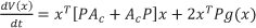
where matrix P is a definite positive matrix. The derivative of V(x) is given by the following expression:

$\frac{dV\left(x\right)}{dt}=x^T\left[P{A}_c+A_{c}P\right]x+2x^{T}Pg(x)$

(37)

Using the Cauchy-Schwarz inequality [18] and inequality (34), the following condition is obtained:

$2x^{T}Pg\left(x\right)\le 2\gamma ||Px||||x||$

(38)

Now, using the following algebraic inequality:

$ab<\frac{a^2}{4}+b^2$

(39)

the following relation is derived:

$2x^{T}Pg\left(x\right)\le {\gamma }^2{x}^{T}PPx+x^{T}x$

(40)

finally obtaining:

$\begin{array}{c}\frac{dV\left(x\right)}{dt}\le x^T\left[P{A}_c+A_{c}P\right]x+{\gamma }^2{x}^{T}PPx+x^{T}x\mathrm{ }\\ \le x^T\left[P{A}_c+A_{c}P+{\gamma }^{2}PP+I\right]x\end{array}$

(41)

From the above, we can state that the system is asymptotically stable if the following condition is satisfied:

$P{A}_c+A_{c}P+{\gamma }^{2}PP+I<0$

(42)

Corollary 4.2. The parameter y in Equation (34) can be increased while keeping the system asymptotically stable if the following convex optimization problem is solved:

$minimize\left\{\rho \right\}$

subject to:

$\left[\begin{array}{cc}{A}_0^{T}P-C^T{X}^T+P{A}_0-XC+I& P\\ P& -\rho I\end{array}\right]<0$

(43)

where

$X=PL;\mathrm{ }\rho =\frac{1}{{\gamma }^2};\mathrm{ }L=\left[\begin{array}{cc}0& 0\\ K_p& K_v\end{array}\right]$

Proof:

To prove the corollary it is necessary to start from the

$P{A}_c+A_{c}P+{\gamma }^{2}PP+I<0$

(44)

This equation, according to the above theorem, guarantees the preservation of the asymptotic stability. Now, representing the matrix A_c as follows:

$A_c=A_0-LC$

(45)

where:

$A_0=\left[\begin{array}{cc}0& I\\ 0& 0\end{array}\right];\mathrm{ }L=\left[\begin{array}{cc}0& 0\\ K_p& K_v\end{array}\right];\mathrm{ }C=\left[\begin{array}{cc}{I}_n& 0\\ 0& I_n\end{array}\right]$

the following equation is obtained:

$P\left(A_0-LC\right)+{(A_0-LC)}^{T}P+{\gamma }^{2}PP+I<0$

(46)

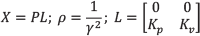
If X = PL, then

$P{A}_0-XC+{A_0^{T}P-C}^T{X}^T+{\gamma }^{2}PP+I<0$

(47)

This matrix inequality is quadratic with respect to P and linear with respect to X, making it possible to show the convexity of the inequality with respect to P and X for a given γ. Now, applying the Schur complement for matrices:

$\left[\begin{array}{cc}A& B\\ C& D\end{array}\right]>0\iff A-B{D}^{-1}C>0\mathrm{ }and\mathrm{ }D>0$

(48)

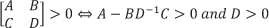
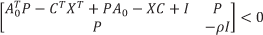
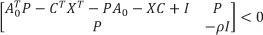
the following matrix inequality is obtained:

$\left[\begin{array}{cc}{A_0^{T}P-C}^T{X}^T-P{A}_0-XC+I& P\\ P& -\frac{1}{{\gamma }^2}I\end{array}\right]<0$

(49)

Finally, defining the value of ρ = −1/γ² yields the following matrix equation:

$\left[\begin{array}{cc}{A_0^{T}P-C}^T{X}^T-P{A}_0-XC+I& P\\ P& -\rho I\end{array}\right]<0$

(50)

From the definition of ρit can be seen that maximizing the value of γ is equivalent to minimizing the value of ρ. The problem can therefore be stated as:

$minimize\left\{\rho \right\}$

subject to:

$\left[\begin{array}{cc}{A}_0^{T}P-C^T{X}^T+P{A}_0-XC+I& P\\ P& -\rho I\end{array}\right]<0$

For a given ρ, the above inequality is affine with respect to the parameters P and X; therefore, the solution can be calculated using convex optimization techniques based on LMI. Also, this solution can be implemented with the aid of computational languages such as Matlab. It is worth noting that the calculation performed to maximize γ does not directly depend on the dynamic model of the robot, because the elements of the matrix A_c are the controller parameters K_p and K_v, which can be modified themselves to maximize the parameter y. This is possible because the uncertainty that exists between the nominal model used by the control law and the real model of manipulator robot was completely transferred to the function g(x). Accordingly, when the upper bound value is increased by manipulating the parameters K_p and K_v, the robustness margin of the closed loop system increases too. Then, applying Matlab toolboxes to solve the convex optimization problem, it is determined that the solution is to assign the eigenvalues of A_c, all real, in the same position, and of course negatives. Thus, the more negative the eigenvalues of A_c are (away from the imaginary axis), the more the robustness margin y increases. However, placing the poles so far away from the imaginary axis results in high controller gains, which is not always desirable because not only does disturbance rejection increase, but also the noise in the measurement sensor is amplified. Fortunately, this problem can be solved by defining a minimum bound to stop the algorithm. This option is defined as (TARGET) in Matlab; it allows the solution of the problem stated in Corollary 4.2. Next, numerical results obtained from simulating a manipulator robot with two degrees of freedom while applying this methodology are presented.

5. Simulations

The method was applied to the case of a planar robot presented in [19], shown in Figure 1.

Figure 1.

Two-joint SCARA-type robot manipulator.

Figure 2.

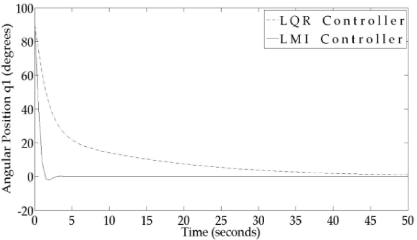
Transient response for q₁ with m_L = 20

Figure 3.

Transient response for q₂ with m_L = 20

The manipulator has the following mathematical model:

$D\left(q\right)\ddot{q}+H\left(q,\dot{q}\right)=\tau$

(51)

$D\left(q\right)=\left[\begin{array}{cc}{d}_{11}& d_{12}\\ d_{21}& d_{22}\end{array}\right],\mathrm{ }H\left(q,\dot{q}\right)=\left[\begin{array}{c}{V}_1+U_1+W_1\\ V_2+U_2+W_2\end{array}\right]$

(52)

and its elements are:

$\begin{array}{l}{d}_{11}=562.0+171.6\cos \left(q_1\right)+100m_L+96m_L\cos \left(q_2\right)\\ d_{12}=51.2+85.8\cos \left(q_2\right)+36m_L+48m_L\cos \left(q_2\right)\\ d_{21}=d_{12}\\ d_{22}=51.2+36m_L\\ V_1=\left(85.8+48m_L\right)\left(2{\dot{q}}_1-{\dot{q}}_2\right){\dot{q}}_2\mathrm{s}\mathrm{i}\mathrm{n}\left(q_2\right)\\ V_2=\left(85.8+48m_L\right){\dot{q}}_1^{2}sin\left(q_2\right)\\ U_1=-20{\dot{q}}_1\\ U_2=50{\dot{q}}_2\\ W_1=\left(820.68+78.4m_L\right)\sin \left(q_1\right)+\\ (105.1+58.8m_L)\mathrm{s}\mathrm{i}\mathrm{n}(q_1+q_2)\\ W_2=(105.1+58.8m_L)\mathrm{s}\mathrm{i}\mathrm{n}(q_1+q_2)\end{array}$

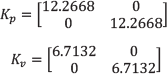
where m_L represents the mass of the object to be moved with the manipulator, which, in practice, may change in value. In this work, as in [19], the mass is considered to be an uncertain value represented by the following range of values: m_L ∈ [4,22] considering m_L = 20 as the nominal value. Using the Matlab LMI toolbox, the following controller parameters are obtained:

$\begin{array}{c}{K}_p=\left[\begin{array}{cc}12.2668& 0\\ 0& 12.2668\end{array}\right]\\ K_v=\left[\begin{array}{cc}6.7132& 0\\ 0& 6.7132\end{array}\right]\end{array}$

(53)

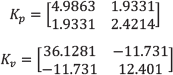
In [19], using LQR optimal control techniques, the following parameters were calculated:

$\begin{array}{c}{K}_p=\left[\begin{array}{cc}4.9863& 1.9331\\ 1.9331& 2.4214\end{array}\right]\\ K_v=\left[\begin{array}{cc}36.1281& -11.731\\ -11.731& 12.401\end{array}\right]\end{array}$

(54)

These parameters, defined in (38) and (39), are substituted into the control law (12); the following simulation results can then be obtained:

Figure 4.

Transient response for q₁ with m_L = 15

Figure 5.

Transient response for q₂ with m_L = 15

Figure 6.

Transient response for q₁ with m_L = 4

Figure 7.

Transient response for q₂ with m_L = 4

Figure 8.

Transient response for q₂ with m_L = 21

Figure 9.

Transient response for q₂ with m_L = 21

Figure 10.

Transient response for q₂ with m_L = 21.8

Figure 11.

Transient response for q₂ with m_L = 21.8

As observed in the previous simulations, the closed loop control system for the robot manipulator performs better despite the uncertainty of the mass of the load when using the control law proposed in this research, mainly when this is bigger than its nominal value. This is logical because it is easier to move something light than something heavier.

6. Conclusions

This paper presented a new tuning method for a special control law to guarantee an increase in the robustness margin of the closed loop system of a robot manipulator based on its mathematical model. The control strategy consisted in transforming the original problem into a convex optimization problem, in order to use a methodology known as LMI to solve it. The results were validated by performing numerical simulations and then using a comparison to show the inferior performance of LQR optimal control techniques. An idea for future research would be to apply the technique presented in this paper to other types of robots, such as Unmanned Aerial Vehicles (UAVs).