
Abstract
This paper focuses on the kinematics, kinetostatics and design optimization of a 2-DOF cable-driven flexible joint module. Based on the motion characteristics of the 2-DOF joint module, the concept of instantaneous screw axis in conjunction with the Product-Of-Exponentials (POE) formula is proposed to formulate its kinematic model. However, as the instantaneous screw axis is unfixed, the Lie group method is employed to derive the instantaneous kinematic model of the joint module. In order to generate the feasible workspace subject to positive tension constraint, the kinetostatics of the joint module is addressed, where the stiffness resulting from both the driving cables and the flexible backbone are considered. A numerical orientation workspace evaluation method is proposed based on an equi-volumetric partition in its parametric space and the volume-element associated integral factor. A global singular value (GSV) index, which considers the minimum singular value of the stiffness matrix of joint module over the achievable workspace, is employed to optimize the geometric size of joint module. The simulation results demonstrate the effectiveness of the proposed GSV optimization algorithm.
Keywords
1. Introduction
The flexible Snake-Like Robot Arm (SLRA) with hyper-redundant Degrees Of Freedom (DOF) is especially suitable for the industrial applications requiring high manoeuvrability over complex and confined spaces such as on-wing inspection and repair of airplanes [1] and search and rescue in collapsed buildings [2]. The Cable-Driven Snake-like Robot Arm (CDSLRA) with a flexible backbone is a promising candidate in the SLRA design, and has received increasing attention in the literature [1, 3, 4].
In this work, a hyper-redundant CDSLRA that consists of a large number of 2-DOF flexible joint modules is to be developed for airplane on-wing inspection and repair applications. In order to improve the performance of the CDSLRA, design optimization of the 2-DOF cable-driven joint module with a flexible backbone becomes a very critical issue, which, however, has not been well-addressed due to the lack of effective kinematics, kinetostatics and workspace analysis models.
In previous efforts, the D-H notation in conjunction with the Euler angles has been extensively employed for the kinematic modelling of a 2-DOF cable-driven joint module with a flexible backbone [3, 4]. However, such a modelling approach could not clearly describe the actual motion characteristics of the module. For example, to represent the 2-DOF bending motions using Euler angles, three sequential rotations (Rz(α)Ry(θ)Rz(-α)) are needed in order to remove the twisting motion about the backbone, although only two Euler angles (α and θ) are used. To avoid such a problem, the instantaneous screw axis concept is proposed in this paper such that the 2-DOF bending motion of the joint module can be clearly described by one rotation about an instantaneous screw axis with its directional component parallel to the x-y plane of the base frame. With such a geometrically meaningful concept, the POE formula [5] can be employed to formulate the kinematic models of the 2-DOF joint module, making the analysis significantly simplified. The proposed kinematic model can also be applied to other types of mechanisms with flexible backbones including the CDSLRA in [1, 3, 4] and air-muscles driven SLRA in [6]. However, for the instantaneous kinematics (velocity) analysis, the instantaneous screw axis needs to be considered as a variable rotation axis. As a result, the conventional instantaneous kinematics formulation approaches based on the fixed rotation axis cannot be employed. In this work, the Lie bracket method [7–10] is employed to analytically derive the manipulator Jacobian of the 2-DOF joint module. Based on the manipulator Jacobian of the 2-DOF joint module, an instantaneous kinematics model is derived for the joint module, which will be used in the following analysis.
Some research efforts exist in the literature analysing the workspace quantity and quality based on the kinematics and kinetostatics properties of the mechanisms, e.g., the workspace volume [11], the global dexterity [12] and the global stiffness analyses [13]. The design optimization of the 2-DOF cable-driven joint module is to achieve a high stiffness performance over the workspace. As a result, a Global Singular Value (GSV) index has been proposed by taking the minimum singular value of the stiffness matrix over the attainable workspace into account. The effectiveness of the proposed optimization algorithm will be demonstrated by simulation examples.
2. Kinematics Analysis of a 2-DOF Cable-Driven Joint Module with a Flexible Backbone
2.1 Design Consideration
The proposed CDSLRA adopts a modular design approach, which consists of a number of serially connected identical 2-DOF cable-driven joint modules. As shown in Figure 1(a), each module comprises a base disk, three cables, an elastic backbone and a moving platform. The moving platform is linked to the base disk through three driving cables and a flexible backbone at the centre of the joint module. To further simplify the joint module design with inter-changeable connectivity among the modules, both the moving platform and the base disk are identical to each other. The attachment points of three driving cables are equally spaced at 120° on both the moving platform and the base disk. Stainless steel cables are employed instead of super-elastic Ni-Ti tubes [4] because the latter have limited driving force.

2-DOF cable-driven joint module
2.2 Joint Module Displacement Analysis
The flexible backbone is made of elastic and inextensible material, and it is designed to be rigid in torsion. Hence, the joint module with such a flexible backbone only allows a two-DOF bending motion, which can be described by two kinematic parameters: rotation angle of the bending plane α and the bending angle θ, as shown in Figure 2.

The kinematics diagram of the 2-DOF joint module
The purpose of the forward displacement analysis is to find the pose of the moving platform T(l)∈SE(3) when the lengths of the three driving cables l=[lc1 lc2 lc3]T are given. Since it is difficult to derive T(l) directly, joint variables φ=[α θ] are used as the intermediate variables to simplify the analysis.
Frame {j-1} is attached to the base disk with its origin located at the centre of the disk, as shown in Figure 1(b).
The zj-1 axis is normal to the disk and the xj-1 axis points to the first cable attachment point on the disk. Similarly, Frame {j} is attached to the moving platform with its origin located at the centre of the platform. The zj axis is normal to the platform and the xj axis points to the first cable attachment point on the platform.
2.2.1 Relationship between joint variables and cable lengths
As shown in Figure 2, Bi and Pi (i=1, 2, 3) are the ith cable attachment points on the base disk and the moving platform respectively. Based on the 2-DOF bending characteristics, the bending shape of the backbone is assumed to be circular with a constant arc length L [3, 4]. The plane OCPB formed by zj-1 and zj, as well as the flexible backbone arc OC is the bending plane, which is always perpendicular to the base disk plane. Point B and P are the intersection points of the bending plane with the base disk and the moving platform respectively. Note that B and P are located on the same circles formed by Bi and Pi (i = 1, 2, 3) respectively. The backbone deflection within the bending plane is described by the bending angle θ(i.e, ∠BMP), while the bending plane is defined by a rotation angle α (∠B1OB).
The length of

where
Here, r is the constant radius from O to B and also from C to Pi. βi is a right-handed rotation angle from

Therefore, for a set of given joint variables α and θ, the cable lengths are determined as follows:

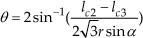
While for a set of given cable lengths, the joint variables can be expressed as:

2.2.2 Determination of kinematics transformation matrix
Denote the forward kinematics transformation from the frame {j-1} to {j} as T(j-1),j∈SE(3), which has the following general form:
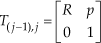
where R∈SO(3) and p∈R3×1 represent the orientation and position of frame {j} with respect to frame {j-1}, respectively. As shown in Figure 2, when the joint variables α and θ are known, the position vector of point C, i.e., p (

However, to determine the orientation of frame {j} with respect to frame {j-1}, i.e., R is not so straightforward. Conventionally, the rotation matrix R is computed through the Z-Y-Z Euler angles as follows [4]:

where sα=sinα, cα=cosα, sθ=sinθ, cθ=cosθ and vθ=1-cosθ.
By analysing the rotation matrix R=[rij]∈SO(3) (i, j =1, 2, 3), we find that r12= r21, r13=-r31, r23= r32.
On the other hand, for a given R∈SO(3), it can always be represented by a rotation about an axis ω=[ω1 ω2 ω3]T ∈R3 (|ω|=1) of a angle θ ∈ R such that [5]

Comparing corresponding terms in (7) and (8), the rotation axis is given by:

Equation (9) implies that the motion of the 2-DOF joint module to achieve a desired posture is equivalent to a rotation about an axis ω that is parallel to the xj-1-yj-1 plane as shown in Figure 3. It can be readily verified that the rotation axis ω is given by the cross product of zj-1 and zj, and the rotation angle is identical to the bending angle θ.
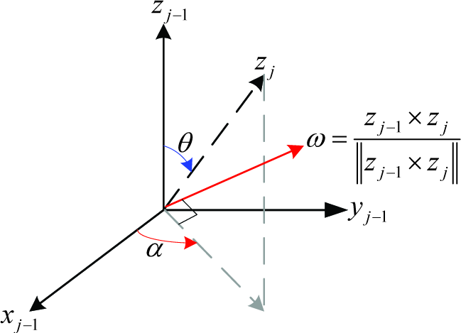
The rotation motion of the 2-DOF joint module
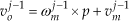
With such a meaningful geometric description, the kinematic transformation of the 2-DOF joint module can be represented by a rotation about an instantaneous screw axis (i.e., a twist),
After such a geometric treatment, the POE formula can be employed to formulate the kinematics models of the 2-DOF joint module.
2.2.3 POE Formula for Forward Displacement Analysis
Based on the screw theory, Murray et al. [5] showed that each rigid motion associated with rotating and translating along the twist direction can be expressed by the product of matrix exponentials. Because of its compact representation and its connection with Lie groups and Lie algebras, the POE formula has proven to be a useful modelling tool in robot kinematics [14, 15]. These advantages make POE formula a convenient and powerful modelling method for hyper-redundant robots.
Based on the POE formula, the forward kinematics of the 2-DOF joint module is given by:

where T(j-1), j(θ,α)∈SE(3) is the final configuration of frame {j} relative to the frame {j-1} as a function of the joint angles θ and α. T(j-1),j(0)∈SE(3) is the initial configuration of frame {j} relative to the frame {j-1} at θ=0 and α=0.

From (10),

Substituting (8) and (9) into (11), and substituting (5) into (12) respectively, then by equating (11) and (12) yields

There are many possible points q on the axis ω, of particular interest is the intersection point between axis ω and the bending plane OCPB, qs, which is expressed by:

where qxy and qz are the projection of vector
Because v = -ω×q, combining (9), (13) and (14) yields

According to (15), it is seen that the point qs on the axis is located on the bisector of ∠PWB, and the height of qs is always equal to L/2, as seen in Figure 4.

Location of point qs on the instantaneous screw axis ω
In brief, the motion of the 2-DOF flexible joint module is equivalent to a rigid body rotation about an instantaneous screw axis
2.3 Joint Module Velocity Analysis
In this section, the velocity analysis of joint module is carried out in order to obtain the Jacobian matrix Jxφ and JIφ.
Since T(j-1), j represents the forward kinematic mapping of the joint module, the instantaneous spatial velocity of the moving platform is therefore given by the twist [5]:

where

vj-1 m ∈ ℜ3×1 denotes the linear velocity of joint module j with respect to frame {j-1}.
Since the instantaneous screw axis

Substituting (18) into (16) yields,

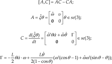
According to the Lie group theory, the right hand side of (19) can be expressed in terms of an infinite series of nested Lie brackets [7–10].
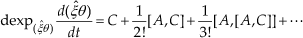
where
ω′ = [-cos α –sin α 0]T is the derivative of ω with respect to α.
Since


According to (21) and (22), the nested Lie bracket in (20) can be simplified. Here only the first four simplified terms of the Lie bracket are listed.


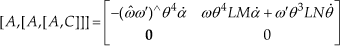
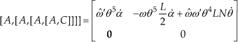
where
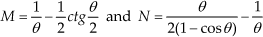
Substituting (23–26) into (20) forms the trigonometric series for the corresponding entries of matrix of


Furthermore, the linear velocity of the origin of the moving platform frame is:
Hence, the velocity of the centre of the moving platform is given by:

where
Combining (27–30) yields the Jacobian matrix as shown in the Equation (31).
Note that the Jacobian matrix in (31) is ill-conditioned when θ = 0, i.e., there is neither bending of the backbone nor rotation of the platform. This singularity at the configuration θ = 0 can be resolved by applying the L'Hopital Rule [3,4].

The instantaneous inverse kinematics can be given as:

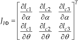
where Jacobian matrix Jlφ is obtained by taking the derivative of (2) for α, θ [3, 4]:
3. Kinetostatics Analysis
3.1 Tension Analysis
The principle of virtual work [4] is employed for the large-deflection beam analysis of the flexible backbone, as obtaining an analytical solution for a large-deflection beam [16] using conventional Newton methods by elliptic integral will be difficult and is unnecessary.
In the following analysis, twisting and extension of the backbone are neglected. Since the backbone is made of linearly elastic material and the bending shape of backbone is assumed to be circular, the strain energy of the flexible backbone is given by [17]:

The virtual work resulting from the infinitesimal joint displacement dφ of the flexible backbone is ∇ETdφ. ∇E represents the gradient of strain energy with respect to joint displacement dφ=[dθ dα]T. Let We=[feT me T]T represents the vector of external forces and moments applied to the moving platform. The virtual work contributed by an infinitesimal displacement dx of the moving platform is WeT dx. If the cable tension to maintain an equilibrium is τ=[τ1 τ2 τ3]
T
, the virtual work done by an infinitesimal displacement dl of the cables is τT dl. By using the principle of virtual work, we obtain:

Substituting (30) and (32) into (35) yields

Therefore, the null space solution of τ is:

where (JlφT)+ = (JlφT)T[(JlφT)(JlφT)T]−1

Using the Cramer's rule, the null vector N of Jacobian matrix JlφT can be written as N={n1 n2 n3}T, in which ni (i=1, 2, 3) is the determinant of the matrix formed by deleting the ith column of the Jacobian matrix JlφT. λ is an arbitrarily scalar.
3.2 Stiffness Analysis
When a CDSLRA performs a given task, an external force and moment vector will be applied on the moving platform. This contact wrench will cause the platform to elastically deviate from its desired motion. The amount of displacement or deformation will depend on both the magnitude of external wrench and the stiffness of the manipulator [18]. Here, we focus on the stiffness model of the 2-DOF joint module of CDSLRA, which is expressed as:

where
The stiffness matrix is symmetric, positive semi-definite and configuration dependent. Equation (38) is derived as follows. By substituting (30), (32) into (35), we obtain

Let δWe∈ℜn represent the change of applied wrench and δx the corresponding displacement changes of the moving platform. We have

where K is the Cartesian stiffness matrix [19] of the joint module.
With (39) and (40), and following the chain rule, we have

As cables behave as linear springs [19], the stiffness equation in the joint space is given as:

where kc = k' diag (l1-1, l2-1, …, lm−1) and k' is the stiffness per reciprocal unit length of cable which is a constant and li is the cable length at a particular pose.

Substituting (30), (32), (42) and (43) into (41) yields (38).
In this paper, the flexible backbone uses a spring steel rod with the diameter db=4mm and Young's modulus E=210GPa. The stainless steel cable is employed and its stiffness per reciprocal unit cable length is k' = 1×10⁵ N/m.
4. Design Optimization
In this section, the design optimization of the 2-DOF flexible joint module is carried out based on workspace quantity and workspace quality. For the workspace quantity, a numerical orientation workspace evaluation method is proposed by using an equi-volumetric partition in its parametric space. Then, in order to achieve a high stiffness quality over the workspace, a GSV, which accounts for the minimum singular value of the stiffness matrix of joint module over the achievable workspace, is employed to optimize the joint module.
4.1 Quantitative Measure
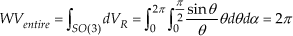
The orientation workspace of the 2-DOF joint module is a subset of the rotation group SO(3). It can be visualized as a circular area in its parametric domain when the polar coordinates are employed to represent the two rotation angles θ ∈ [0,π/2] and α∈[0,2π], as shown in Figure 5. However, the orientation workspace volume of the 2-DOF joint module as described in SO(3) (VSO(3)) is not equal to the geometrical volume of the circular area in its parametric domain due to the nonlinear parameterization. Therefore, an integral factor has to be introduced, which is orientation dependent. For the polar coordinate parameterization, it has been shown that the integration factor is given by sinθ/θ [20]. Hence, the maximum orientation workspace volume of the 2-DOF joint module is given by:
Equi-volumetric partition of a circular area in polar coordinate
To evaluate the orientation workspace volume for a particular 2-DOF joint module, a numerical analysis approach that can generally cope with complicated workspace boundaries (due to the mechanical constraints and singularities) is more effective. Hence, a finite partition of the orientation workspace in its parametric domain is necessary. Similar to [11], the parametric domain of two rotation angles θ and α in the polar coordinate can be partitioned into 3n2 finite elements with equal volume, as shown in Figure 5. When a double index (j, k) is specified for an element, the coordinates of the feature points can be readily computed. Using Equation (44), the orientation workspace for a subset of rotations S ∈ SO(3) can be numerically computed as:

where θjk =πj/2n, αjk=2nk/(6j-3), Vt=π3/12n2 is the element's volume in its parametric domain for the equi-volumetric partition scheme. In this paper, the number of division n=50.
4.2 Qualitative Measure
Displacement or deformation on the moving platform will emerge if an external wrench is applied to it. This deformation depends on both the external wrench and the stiffness of the manipulator. Thus the stiffness has effect on the position accuracy of the manipulator. Also, the 2-DOF cable-driven joint module with the flexible backbone structure has a relatively low stiffness. Therefore, it is necessary to evaluate the stiffness quality over the entire attainable workspace so as to attain an optimal design with a high stiffness performance.
Since the stiffness matrix K of the joint module relates the applied external wrench We on the moving platform to the moving platform deformation x, from the singular value decomposition theorem [21–22], the bounds on |x| can be established as

where σmax and σmin are the maximum and minimum singular value of the stiffness matrix of the joint module. They give the lower and upper bounds of the deformation | x | on the moving platform.
Supposing the vector We is unity, i.e., | We | =1, then the minimum and maximum deformations can be obtained as
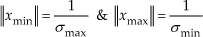
Thus, 1/σmax and 1/σmin are actually the minimum and maximum deformation on the moving platform when the external wrench are unity. Furthermore, the deformations form a deformation ellipsoid, whose axes are directed along the left-hand singular vectors of the pseudo-inverse of the stiffness matrix K+. Its magnitudes are all the singular value of K+. The minimum and maximum deformations in (47) are in the direction of the minor and major axis of the ellipsoid. Normally, the smaller the maximum deformation, the better the stiffness performance, and this maximum deformation bound depends on the σmin. Therefore, the minimum singular value σmin is usually used as the criterion to design the manipulator with respect to its the stiffness [23–24]. Moreover, a larger σmin can lead to a smaller deformation, i.e., better stiffness performance.
Since the stiffness matrix is configuration-dependent, based on (47), the GSV index, which can evaluate the stiffness characteristics of the joint module over the achievable workspace, is defined as

where ha is the sum of all the achievable workspace volume elements. σri min is the minimum singular value of the stiffness matrix K at the specified posture i. Normally, the index value GSV is expected to be as large as possible.
4.3 Design Optimization
4.3.1 Decision Variables
For the design optimization of the 2-DOF joint module, the decision variable kl is the ratio of the radius of the base disk to the length of the backbone, i.e., kl=r/L (0≤k1≤1), which is a very critical design parameter. In this paper, the backbone length L is set to be one unit length.
4.3.2 Constraints
For a cable-driven mechanism, the tension of the cables is required to be positive in order to fully constrain the moving platform. Therefore, the GSV of the joint module can be determined by checking the tension conditions of three cables using the tension analysis. It is seen that the tension solution τi in the Equation (37) can always be made positive for all positive homogeneous solutions regardless of the value of D. This is achieved by changing the arbitrarily scalar λ to compensate the particular solution. The boundary of the workspace can therefore be purely based on the null vector N. Hence, the design constraints for positive cable tension are given as follows [25]:
4.4 Optimization Results
The r/L-GSV relationship is plotted in the Figure 6. It is shown that for the joint module with decision variable r/L∈[0.06,0.637], the GSV is proportional to r/L. This means that a larger ratio r/L can lead to a larger GSV index, i.e., better stiffness performance. The largest GSV=581.3767 is obtained when r/L=0.637. Furthermore, the attainable workspace volume of the joint module is 6.1119 radians, which is very close to the maximum orientation workspace volume (2π), as shown in Figure 7. It is observable that there are three blank spaces (radial strips) inside the circular area, which indicates that the workspace cannot be attained when the rotation angle α=0, 2π/3 and 4π/3, where the positive tension constraint cannot be satisfied.

r/L-GSV relationship plot

Orientation workspace in polar coordinate GSV-based optimized
5. Conclusion
In this paper, the critical kinematic and kinetostatic modelling and analysis issues pertaining to the design optimization of a 2-DOF joint module with a flexible backbone are discussed. It has been shown that the 2-DOF bending motion of the flexible joint module can be represented by a rotation about an instantaneous screw axis, which significantly simplifies the kinematics analysis. Furthermore, utilizing the Lie bracket method from the group theory, the instantaneous kinematic model has been formulated for the 2-DOF joint module. An effective orientation workspace evaluation method is proposed based on an equi-volumetric partition in its parametric domain. The stiffness model of the joint module is formulated, which includes those contributed by both the cables and the flexible backbone. A global singular value (GSV) index, which considers the minimum singular value of the stiffness matrix of joint module over the achievable workspace, is employed to optimize the joint module. The effectiveness of the proposed optimization algorithm is demonstrated through a simulation example.