
Abstract
This work describes neural network training techniques for enhancing the performance of a one-dimensional beam for determining load positions. The system was a distributive system which relied on the detection of changes in the surface properties that can be seen across the surface. The demonstrated distributive system was 400 mm in length. The applied load positions within the range 60–300 mm could be determined with an average percentage error of 0.2% of the beam length which corresponded to a position error of 0.8 mm using a network trained with 10 training positions. It was found that the errors were higher for the load applied near the edges of the beam, leading to an average percentage error of 3.6% for the whole length of the beam. The normalization of the network output can be employed to reduce the average percentage error by approximately 1% for a given number of training positions. The performance was improved by introducing more training positions in the less sensitive area. The described training technique not only reduced the prediction error but also enlarged the areas where the prediction errors were satisfactorily small. Using the described technique, the overall prediction error could be decreased by 0.13–0.24% of the beam length for 30–10 training positions.
The area where the prediction errors were within 2 mm was increased by 14.5–7.3% of the beam length for a network trained with 4 training positions in the middle portion using 10–30 training positions.
1. Introduction
Mechanical interaction is essential for a robot to achieve similar results to humans in an unstructured environment. A robot may be required to make physical contact with an object for manipulation purposes and estimations of hardness, weight, size, position, roughness, stiffness and thermal properties. Although other stimuli can be used to provide the state of contact, force measurement remains the fundamental element as the force data can be easily interpreted and related to other contact parameters. The research area for obtaining information of an object through mechanical interaction is referred to as tactile sensing.
Current applications of tactile sensing in robotics include identifying physical properties and manipulation. Tactile sensing is also employed to enhance vision sensing in establishing the properties of an object. When integrated with a robot finger or multiple fingers, tactile sensing can be devised to measure grasped object profiles [1–3], identify object materials [4] and determine contacting load and location [5]. Some applications have been devised for controlling and manipulating grasped objects; for example, devices for detecting slip [6–8]. Brett and Stone [9] and Evans and Brett [10] examined an approach to determine a contact with soft objects and for adjusting a grasping strategy to control deformation. Flat surfaces with array sensors are the focus of several studies on emulating vision systems for the discrimination of two-dimensional [11] and three-dimensional objects [12–13]. Tactile sensors for discriminating material properties [14] and for detecting thermal properties [15] are also available. Applications of tactile sensing in medicine are emerging and are currently receiving significant attention. A number of research studies on medical tools for force feedback for surgeons in minimal access therapy are currently in progress [9, 16–17]. More examples of tactile systems can be obtained from Lee and Nicholls [18], which provides an extensive collection of works on tactile systems in the 1990s. Yousef et al. [19] reviewed the state-of-the-art in force and tactile sensing technologies that might be suitable within the specific context of dexterous in-hand manipulation. An extensive review on the development of tactile sensing including transduction techniques, past trends and advancements as well as future trends has been discussed by Tiwana et al. [20].
A distributive sensor consists of multiple sensing elements arranged in a linear or two-dimensional array. The derivation of contact relies on the relative information obtained at individual sensory locations to create a “signature” or “pattern” which differs from one contact type to another. In other words, a distributive sensor requires the coupling effect between sensing elements. This is a unique characteristic of a distributive tactile sensor that distinguishes it from most array-type sensors that address the isolation of individual sensing sites from the entire array in the construction. A distributive tactile sensor can be realized through an appropriate selection of contacting surface, substrate and sensing elements. The resolution of a distributive device depends upon the interpretation algorithm rather than the number of sensing elements. As a result, a distributive system has the advantage of having higher spatial resolution than an array sensor with the same number of sensing elements. It should be noted that the regions between two sensing elements of an array sensor that have no sensitivity are sometimes referred to as dead areas [21] while this is not the case with distributive tactile sensors. Brett and Li [22] demonstrated that the dead areas of distributive sensors did not depend upon the number of sensing elements, but rather on the interpretation algorithm.
The distributive approach has previously been successfully used for tactile sensing and in order to sense contact force distribution in gripping devices. Mathematical algorithms have been shown to be important for improving the performance of distributive tactile sensors. Ellis et al. [23] and Stone and Brett [24] used an early version of the distributive technique, using closed-form interpretation algorithms to derive contact force information from the sensory data. Ma et al. [25] discussed the development of a flexible digit with tactile feedback in applications of minimally invasive surgery. Elliott et al. [26] described the use of a distributive tactile sensor to track the position of an unknown moving load along a plate. In their work, neural networks were used to determine the contact and a genetic algorithm was used to optimize the sensing positions and Karhunen-Loeve decomposition for data dimensionality reduction. In a more closely related application, Tongpadungrod et al. [27] used the distributive sensing method to determine the position of a static force on a one-dimensional surface. The paper described a method to optimize the sensing positions of a simple one-dimensional distributive tactile sensing surface using principal component analysis (PCA) as a tool to evaluate optimization performance. Tongpadungrod and Rungrattanaubol [28] showed the effects of the spread of neural network training positions on the prediction performance of a distributive tactile sensor.
This work describes neural network training techniques for enhancing the performance of a distributive tactile sensor for determining the position of a point load. A neural network is used as an algorithm to infer an applied load position from the sensing information obtained from the surface. Three techniques of training the neural network were explored. The first technique was to increase the number of training positions. The second technique was to normalize the network outputs such that they were in the same range as the beam length. The third technique was to introduce more training positions near the beam edges, where they were less sensitive to an applied load. The performances will be compared based upon the prediction errors and the system effective areas.
2. Methodology
2.1 Descriptions of the system for data acquisition
The distributive system used in the case study was defined as a simply supported beam structure. The system was used to determine the position of a constant point load on the contact surface using the beam deflection as input. The arrangement of the system in this study is shown in Figure 1.

The one-dimensional distributive beam system under investigation
The one-dimensional surface was a mild steel beam of dimensions 40 × 400 × 1.2 mm supported at both ends by wedges. A 3 N load with a point contact with the surface was applied on the beam surface. The beam deflection caused by the point load was measured at 8 positions located at an equal pitch of approximately 44 mm across the beam length. The deflection of the beam at the measurement points was generated by simulation, as described in the next section.
2.2 Mathematical model for data acquisition
In order to efficiently study the performances of the investigated system, a mathematical model describing the behaviour of the system was defined and the corresponding computational simulation was developed.
The deflection of the beam surface can be calculated from the standard beam bending theory reported in most structural mechanics texts, for example [29]. For a simply supported beam, the deflection y at position x in response to an applied load W at position a on a simply supported beam of length l is given by:

where E is Young's modulus and I is the second moment of the area. For equation (1), the following assumptions are applied: (a) the beam is straight, (b) the beam is constructed from a homogeneous material of constant elasticity, (c) the cross-sectional area remains planar and is uniform, (d) the applied load will not cause permanent deformation, and (e) any deflections are small with respect to length.
A simulated beam deflection was used throughout this study based on the principle of beam deflection described by equation (1). The load W was fixed at 3 N, the beam length l was 400 mm and Young's modulus E was 200 MPa. The second moment of area I was calculated from a beam dimension of 40 × 1.2 mm. In this study, the deflection y was calculated at 8 points of measurement x at a pitch of 44.4 mm. The load position a was the parameter that the system was used to infer from the beam deflection.
2.3 Description of the neural network
To demonstrate the use of distributive tactile sensing, a back propagation neural network was used as an interpretation algorithm. The neural network was employed to illustrate its performance and sensitivity in a distributive tactile sensing system. The neural network used the beam deflection at the measuring points as the inputs in order to determine the corresponding applied load position as the output. Prior to the prediction, the neural network was first used to establish the relationship between the inputs and the outputs using the information from selected load positions that will be referred to as the training positions.
2.3.1 Neural network architecture
The networks consisted of 3 layers: the input layer, the output layer and the hidden layer. The input layer had 8 nodes corresponding to 8 inputs of the beam deflection at the measuring points. The output layer was a single node corresponding to the applied load position. The network output for a predicted load position had a value between 0–1. The hidden layer was between the input and the output layers. In the hidden layer, there were 10 hidden nodes which were mathematically connected to the input and the output nodes. The load positions and the corresponding beam deflections at the points of measurement were fed to the network for training. In the training process, the momentum rate and the learning rate were fixed at 0.9 and 0.7 respectively. The training was carried out to achieve the aggregate error between the desired outputs and the network outputs of no more than 0.001%. The training process came to an end when the aggregate error was within the specified limit or else it was terminated when the number of iterations exceeded 106 iterations.
2.3.2 Equally-spaced training positions
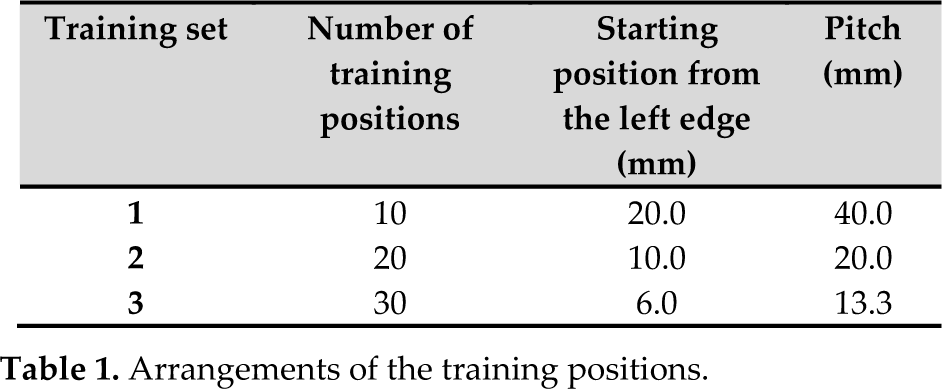
Three sets of training data with 10, 20 and 30 training positions were explored. The training positions were at an equal pitch, depending upon the number of training positions. The arrangements of the training positions are shown in Table 1.
Arrangements of the training positions.
2.3.3 Types of network output
The neural network output took a value between 0–1. The network output was thereafter converted into the position of an applied load from the left edge of the beam, having a value between 0-400 mm. In this study, two types of network output were examined: position output and normalized output, having the description as follows.
a. Position output
In the first investigation, the network output was the actual load position in meters (0-0.4 m) from the left edge. This will be referred to as the position output. The span of the network output corresponding to the beam length was a value between 0 (load applied on the left edge) and 0.4 (load applied on the right edge). However, the network itself can output a value of up to 1, which corresponds to a load position of 1 m from the left edge. As a result, the network output was allowed to exceed the actual beam length. As an example, a string of training data of the position output for the training position 20 mm (from the left edge) is as follows:

The dotted line area contains the training input (simulated beam deflection) and the solid line area contains the training output (the load position). The string of data consists of 9 elements. The first eight elements within the dotted line rectangle correspond to the beam deflection at the measuring points. The negative sign denotes the deflection in the downward direction. The last element within the solid line rectangle corresponds to the position of an applied load (meter) from the left edge of the beam and has a maximum value of 0.4 (equal to the beam length) in training.
b. Normalized output
The normalized output was defined as the applied load position divided by the beam length. By normalization, the span of the network output corresponding to the beam length was a value between 0 (load applied on the left edge) and 1 (load applied on the right edge). When a trained network was used to determine applied load positions, the output value was multiplied by the beam length to obtain the result of the applied load position. In this way, the predicted applied load position would not exceed the beam length. As an example, a string of the training data of the normalized output for the training position 20 mm (from the left edge) is as follows:

The dotted line area contains the training input (simulated beam deflection) and the solid line area contains the training output (load position). The first eight elements within the dotted line area correspond to the beam deflection at the measuring points. The last element within the solid line rectangle corresponds to the normalized applied load position from the left edge of the beam. The normalized output had a maximum value of 1 (load applied at the right edge). In this way, the maximum network output training value and the maximum prediction value were the same. For this specific example, the last element of the string which corresponded to the applied load position at 20 mm, had increased from 0.02 with the position output to 0.05 with the normalized output as a result of normalization by the beam length of 0.4 m.
2.3.4 Determination of network performance in predicting applied load positions
After the training, the networks were used to determine applied load positions from the deflection at the points of measurement. The performance of each network was studied using test data of 399 load positions at an equal pitch of 1 mm. It should be noted that some of the test data may be the same as the training positions.
In the analyses carried out in the following section, the performance was obtained in terms of the percentage error, which was the positional error as a percent of the beam length [27] calculated from equation (2).

where e is the percentage error of the beam length (%), a is the applied load position (mm), a′ is the predicted load position (mm) and l is the beam length (mm).
3. Results and discussion
In the network training process, strings of training data containing both the beam deflections (the network input) due to load applications at the training positions (the network output) were supplied to the network. The network used the training data to establish mathematical connections between the beam deflections and the load position. The mathematical connections were adjusted until the aggregate difference between the desired load position and the actual network output was within the specified limit of 0.001%.
3.1 Performance of the neural network trained with 10 position outputs
The network was trained with 10 training positions between 20–380 mm from the left edge of the beam. The aggregate error was achieved after 26,850 iterations. After training, the network was tested for its performance for applied load positions from 1–399 mm at a step of 1 mm. The predicted applied load positions were plotted against the actual load position, as shown in Figure 2.

Predicted applied load positions from the network trained with 10 position outputs.
It can be observed that most of the predictions by the network agreed with the actual applied load positions for the load positions in the approximate range between 50–300 mm. Larger errors were illustrated when the load was applied near the edges of the beam. Figure 2 shows that the prediction values overshot 400 mm, which was the length of the beam. This was a result of using an actual load position (in metres) as the network input. The errors at the edges could also be a result of the small input magnitude which corresponded to the small beam deflections when the load was applied near the supports of the beam. In contrast, the load applied near the beam centre caused larger deflections that were more easily identified. The results indicated that the network was less effective near the beam edges outside the training area. On average, the error was 3.6% of the beam length (or 14.4 mm). Within the trained proportion (20–380 mm), the average error was reduced to 1.4% (or 5.4 mm). It was found that all of the individual percentage errors for the length 60–300 mm were less than 0.5% (or 2 mm) with an average of 0.2% (or 0.8 mm). The summary of these errors is shown in Table 2.
Summary of the average percentage errors and the position errors for different proportions of the beam.

This investigation suggested that the system was most effective in the portion 60–300 mm (or 60% of the beam length) where the average position error was less than 2 mm. This portion was within the trained area and distant from the edges. For this arrangement, the space between the measuring points was 44.4 mm while the overall average position error was at most 14.4 mm. The spatial error of the system was smaller than the space between the measuring points. This is an important characteristic of distributive sensors in that the determination of an applied load is made from several sensing elements rather than from local elements near the point of contact.
3.2 Enhancement of the neural network performance by using normalized output
In the training process, the network established the relation between the beam deflection and the applied load position. At the start of the training, the difference between the output and the desired applied load position was high. The difference diminished as the training process progressed until reaching a specified value or else the training process was terminated after some given number of training iterations. This is characteristic of typical behaviour in neural network training. In an attempt to reduce the number of iterations and the percentage errors, the networks trained with the position output and the normalized output were compared. A plot of the number of training positions and the iteration number at which the training reached the specified error is shown in Figure 3.

The number of training iterations as a function of the number of training positions for the networks trained with the position output and the normalized output.
In the training process, all of the networks were successfully trained to reach an aggregate error below 0.001% within 106 iterations. The number of training iterations for the normalized output was smaller compared with the case with the position output at the same number of training positions. The number of training iterations increased with an increase in the number of training positions. For the case of the position output, the increase in training iterations with the number of training positions was linear. In the case of the normalized output, the increase in training iterations between 10–20 training positions was sharp but became gradual between 20–30 training positions. The results showed that the use of normalized output was useful, especially when the neural network requires a large number of iterations to reach the specified accuracy. As for application examples, the normalized output may be used to reduce the number of training iterations when the network is required to establish more complicated load parameters, such as the load distribution on a surface or the dynamic motion of a moving load.
The accuracy of the network in determining applied load positions was evaluated through the percentage errors calculated from equation (2). For the network trained with different numbers of training positions and output methods, the average percentage error for the load positions in the range 1–399 mm from the left edge of the beam was calculated and plotted in Figure 4.
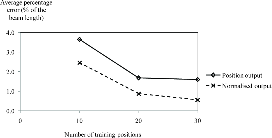
The average percentage errors as a function of the number of training positions for the networks trained with the position output and the normalized output.
As expected, the percentage error decreased with an increase in the number of training positions for all of the cases explored. In the case of the position output, the percentage error decreased from 3.6% to 1.6% of the beam length when the number of training positions increased from 10 to 30 positions. In the case of the normalized output, the percentage error decreased from 2.5% to 0.6% of the beam length when the number of training positions increased from 10 to 30 positions. For both types of outputs, the network became more precise after experiencing more samples of training positions. For a given number of training positions, the network trained with the normalized output had an average percentage error of approximately 1% less than that of the network trained with the position output. For the training with the position output, the output had a span of 0–1 m beyond the beam length of 0–0.4 m. This resulted in an overshoot of the network prediction causing large errors for the applied load positions near the right edge of the beam. The problem was eliminated when using the normalized outputs. For both types of network outputs, the decrease in the percentage error was sharp when the number of the training positions increased from 10 to 20 positions. However, the decrease in the average percentage error became more gradual when the number of the training positions increased from 20 to 30 positions. The number of training positions was close to optimal at 20 positions and only an improvement in accuracy might be expected beyond this point.
3.3 Enhancement of the neural network performance in predicting positions near the edges by the strategic spacing of training positions
When using the equally spaced training positions, the magnitude of the beam deflection diminished as the load position approached the edges of the beam and weakened the neural network's performance. This section discusses a technique to improve system performance by increasing the number of training positions near the edges of the beam. The effects of a change in the number of training positions in the less sensitive areas were examined through the change in the number of the training positions in the middle portion of the beam. The middle portion was defined as the length 100–300 mm from the left end of the beam while the edge areas were the lengths within 100 mm of both sides of the beam supports. The system performance with 10, 20 and 30 training positions with normalized outputs will be compared between (1) equally spaced training positions, (2) 6 training positions in the middle portion, and (3) 4 training positions in the middle portion. For cases (2) and (3), there were 2 fixed training positions in the middle portion at 100 and 300 mm (which were the edges of the middle portion) while the other training positions in the middle portion were equally distributed within the middle portion. Other training positions were divided into two equal sets distributed at an equal pitch in each side of the edge of the beam. The arrangements of the training positions for the equally spaced training positions (training sets 1, 2, and 3) and the performance improvement technique (training sets E1.1, E1.2, E2.1, E2.2, E3.1 and E3.2) are shown in Table 3. The pitch between the training positions was increased in the middle portion since in general there were fewer training positions in the middle portion. The pitches between the training positions in the edge areas of the performance improvement technique were comparatively smaller while the starting positions from the left edge were further to the right-hand side of the beam. As a result, the training positions of the performance improvement technique covered smaller areas compared to the early arrangements with the equally spaced training positions.
Arrangements of the training positions for the performance improvement technique.

The average percentage errors for the load positions in the range 1–399 mm from the left edge of the beam with an increment of 1 mm for the networks trained with the equally spaced training positions and with the performance improvement technique were calculated and plotted in Figure 5.

The average percentage errors as a function of the number of training positions for the networks trained with the normalized outputs for (1) the equally spaced training positions, (2) 6 training positions in the middle portion, and (3) 4 training positions in the middle portion.
With an exception of 10 training positions with 6 training positions in the middle portion, for a given training position the average percentage error of the improvement technique was smaller than that of the equally spaced training positions. The average percentage errors decreased slightly, from 0.57–2.46% to 0.44–2.18% of the beam length with 4 training positions in the middle portion. The prediction errors tended to decrease with the number of training positions in the middle portion - that is, with an increase in the number of training positions in the edge areas.
The highest error appeared in the case of training with 10 positions with 6 positions in the middle portion. This particular case disagreed with the other results. It was possible that the first training position in this case was located at 33.0 mm, which was the furthest from the beam support at the edges while the first training positions of the other cases were not so different. Because the first training position was further from the edge, the system did not experience smaller deflections when the load was close to the edges. The untrained areas near the edges caused large prediction errors. The results in this part suggested that an improvement in the system accuracy could be achieved by strategically locating more training positions near the edge areas (with a smaller number of training positions in the middle portion). The effective length was calculated as a percentage of the beam length and plotted in Figure 6.

The effective lengths as a percentage of the beam length for the networks trained with the normalized outputs for (1) the equally spaced training positions, (2) 6 training positions in the middle portion, and (3) 4 training positions in the middle portion.
The percentage effective lengthswere approximately 63.5–87.5% of the beam length for the network trained with equally spaced training positions, 70.3–94.5% of the beam length for the network trained with 6 training positions in the middle portion, and 78.0–94.8% of the beam length for the network trained with 4 training positions in the middle portion using 10–30 training positions. The effective length increased with the number of training positions for a given training technique. The rate of increase of the effective length slowed down with the number of training positions, suggesting that the effective length approached an optimal point at a certain number of training positions. For a given number of training positions, the training technique with 4 training positions in the middle portion of the beam resulted in the largest effective length for all of the cases explored. The difference between the effective areas of the equally spaced training positions and the performance improvement techniques declined with an increase in the number of training positions.
6. Conclusions
The accuracy in determining the applied load positions can be improved by the neural network training strategies. The described distributive system was able to determine applied load positions using as few as 10 training positions. The error was high for applied load positions near the edges of the beam, but decreased as the load positions moved further from the edges. The performance could be improved by an increase in the number of training positions. The network trained with the normalized output out-performed the network trained with the position output. By using the normalized output, the number of training iterations and the percentage error were both reduced. The strategic spacing with 4 training positions in the middle portion resulted in a reduction in the percentage errors and enlarged the areas where the prediction errors were satisfactorily small. The highlights of the proposed tactile sensing system are its simplicity and its low-cost setup and satisfactory performances. The described algorithm can be integrated with a robot and a feedback system for object manipulation. The technique can be extended to more complicated cases such as two-dimensional systems.
Footnotes
7. Acknowledgements
The author would like to thank the Faculty of Engineering of King Mongkut's University of Technology North Bangkok for the financial support for this work. A special thanks go to Dr. Chantaraporn Phalakornkule for her support and suggestions for this article.